Exploring Quasi-Linear Equation(Arnold’s ODE)

This post is based upon my reading of the section on Quasi-Linear Equation in Arnold’s ODE.

In the previous 2 posts, we looked at linear homogeneous PDE’s:

$a_1(x) \frac{\partial u}{\partial x_1} + ... + a_n(x) \frac{\partial u}{\partial x_n} = 0$ (*)

The characteristic vector field corresponding to (*) is given by:

$\dot{x} = (a_1, ..., a_n)$

This vector field lives in the x-space. Geometrically, the restriction of any solution $u(x)$ to a phase curve of the characteristic vector field is a constant. This is equivalent to saying that the vertical projection of the level lines of the graph of $u(x)$ in the (x, u)-space onto the x-space gives us the phase curves of the characteristic vector field.

We also looked at linear inhomogeneous PDE’s:

$a_1(x) \frac{\partial u}{\partial x_1} + ... + a_n(x) \frac{\partial u}{\partial x_n} = b(x)$

Key: the characteristic vector field no longer lives in the x-space; rather, it lives inside the (x, u)-space, i.e. the space of 0-jets.

The characteristic vector field is given by:

$(\dot{x}, \dot{u}) = (a_1, ..., a_n, b)$

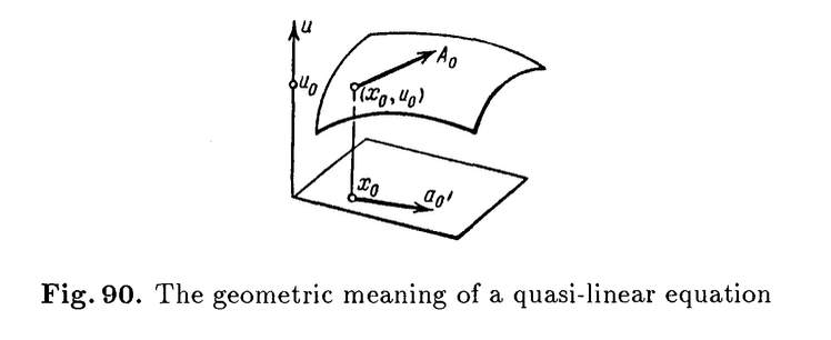
Geometrically, this means that a point $x$ leaves point $x_0$ in the x-space with velocity $(a_1(x_0), ..., a_n(x_0))$ (i.e. a particle is moving along a phase flow of the field $\dot{x} = (a_1, ..., a_n)$ ), then the value of $u(x)$ begins to change with velocity $b(x_0)$ .

Notice: this vector field is invariant under translation along the u-axis. Hence, the vector field is the same for any fixed u-value. The vertical projection of such vector field onto the x-space is well-defined and gives us the vector field $(a_1, ..., a_n)$ that corresponds too the linear homogeneous PDE $a_1(x) \frac{\partial u}{\partial x_1} + ... + a_n \frac{\partial u}{\partial x_n} = 0$ .

Quasi-linear Equation

Now, let’s look at the case where the corresponding vector field not only depends on the x-value but also the u-value, i.e.

$a_1(x, u) \frac{\partial u}{\partial x_1} + ... + a_n(x, u) \frac{\partial u}{\partial x_n} = b(x, u)$ (**)

We can see that the linear inhomogeneous equation is really just a special case of this. The characteristic vector field for (**) is:

$(\dot{x}, \dot{u}) = (a_1(x, u), ..., a_n(x, u), b(x, u))$

and it lives in the (x, u)-space. But in this case, the vector field is no longer invariant under translation along the u-axis. However, the same geometric interpretation still applies.

Example: the motion of one-dimensional medium of particles moving along a line by inertia (velocity of each particle is constant) can be described by a quasi-linear equation.

Let the velocity of the particle at point $x$ at time $t$ be $u(t, x)$ .

Set $x = \phi(t)$ to be the motion of a particle. Then,

$\dot{x} = \dot{\phi} = u(t, \phi(t))$ and

$\ddot{x} = \ddot{\phi} = \frac{d}{dt} u(t, \phi(t)) = \begin{bmatrix} \frac{\partial u}{\partial t} \\ \frac{\partial u}{\partial x} \end{bmatrix} \cdot \begin{bmatrix} \dot{t} \\ \dot{\phi} \end{bmatrix} = \frac{\partial u}{\partial t} + \frac{\partial u}{\partial x} \dot{\phi}$

Since the acceleration of the particle is 0, it follows that:

$\frac{\partial u}{\partial t} + \frac{\partial u}{\partial x} \dot{\phi} = 0$

This is the quasi-linear equation that describes the motion of the particles.

Example 1.a: Construct the graph of the solution at the instant t if $u = arctan(x)$ for $t = 0$ .

Key: the restriction of the characteristic vector field to the (x, u)-plane is

$\dot{x} = u$

$\dot{u} = 0$

Why? Because $\dot{x}$ is the velocity of the particle, which by definition is $u$ ; $\dot{u}$ is the acceleration of the particle, which we know to be zero.

The phase flows of this vector field on the (x, u)-plane is:

$\phi: \tau \mapsto (x + u \tau, u)$

Notice that the family of all phase flows for a fixed time $\tau = \tau_0$ corresponds to a diffeomorphism of the plane, more specifically, a diffeomorphism of the vector field on the plane.

Geometrically, this diffeomorphism $\Psi_{\tau}: (x, u) \mapsto ( x + u \tau, u)$ maps the graph of the solution at the instant 0 to the graph of the solution at the instant $\tau$ .

Given the initial point $(x_0, arctan(x_0))$ , the corresponding point after moving along the phase flow for time $\tau$ is $(x_0 + arctan(x_0)\tau, arctan(x_0))$ .

Thus, for $t = \tau$ , the graph is given by the set:

$\{ (x_0 + \arctan(x_0) \tau, arctan(x_0)) : x_0 \in \mathbb{R} \}$

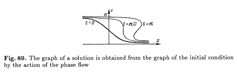
Notice: for $t \geq \pi/2$ , no smooth solution exists.

Example 1.b: Construct the equation for the evolution of the velocity field of a medium of noninteracting particles in a force field with force F(x) at the point x.

Let $u(t, x)$ be the velocity of a particle at time t and position x. Let $\phi(t) = x$ be the motion of the particle. Then,

$\dot{x} = \dot{\phi}(t) = u(t, \phi(t))$ and

$\ddot{x} = F(\phi(t))$ (the force F(x) gives us an acceleration F(x), if we assume the particle to have unit mass)

We also know that $\ddot{x} = \frac{\partial u}{\partial t} + u \frac{\partial u}{\partial x}$ .

Thus, we obtain the equation $\frac{\partial u}{\partial t} + u \frac{\partial u}{\partial x} = F(x)$ .

Example 1.c: Solve this equation with the initial condition $u|_{t=0} = 0$ for the force field $F(x) = -x$ .

Key: we focus on the restriction of the vector field to the (x, u)-plane for a fixed instant of time.

The corresponding vector field is given by:

$\dot{x} = u$

$\dot{u} = -x$ (because the acceleration is $F(x) = -x$ )

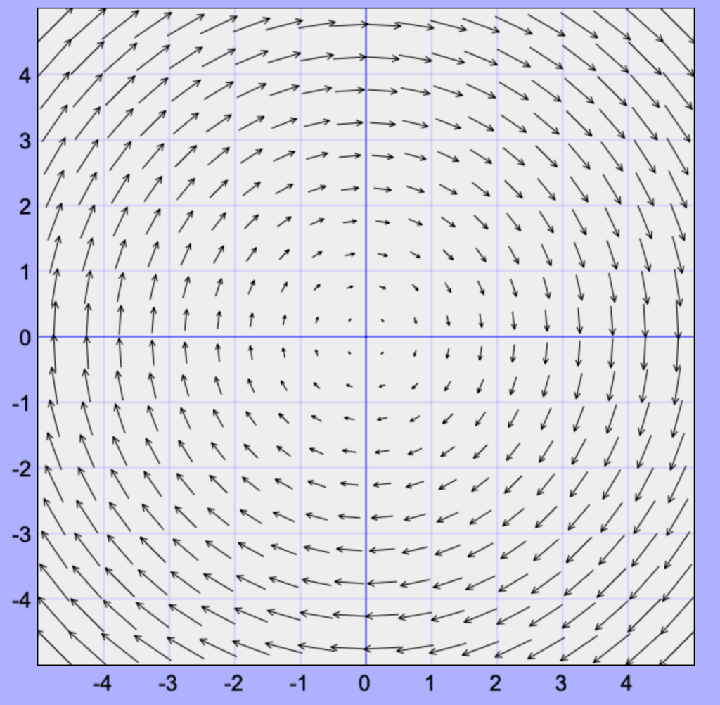
The corresponding phase curves are circles centred at the origin.

The phase flow passing through an arbitrary point $(x_0, u_0)$ is given by $\phi: \tau \mapsto (-cos(\tau) x_0, sin(\tau) u_0)$ .

As given, the graph of the solution at the instant $t = 0$ is the line $u = 0$ . The corresponding graph of the solution at $t = \tau$ is obtained by moving each point on $u = 0$ along the phase flow for time $\tau$ . In this case, this would be rotating the line $u = 0$ by an angle $\tau$ clockwise. The resulting graph is on the (x, u)-plane is $u(t, x) = -x tan(\tau)$ .