Lifting to a Legendrian Curve v.s. Blowing Up at a Point

Recall: from the previous post, the bundle of contact elements on $\mathbb{R}^2$ is $\mathbb{R}^2 \times \mathbb{RP}^1$ .

A contact element on $\mathbb{R}^2$ is a point with a line passing through the point, i.e. $(p, \ell)$ . The bundle of contact elements is the set of space of lines passing through each $p \in \mathbb{R}^2$ . We can also think about this as the extended space of 1-jets, where we also consider the point at infinity along the p-axis.

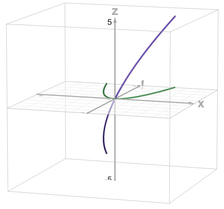
Given a smooth curve, $\mathcal{C}$ , in $\mathbb{R}^2$ , we can look at the corresponding curve, $\tilde{\mathcal{C}}$ , arising from the set of contact elements on $\mathbb{R}^2$ tangent to $\mathcal{C}$ in $\mathbb{R}^2 \times \mathbb{RP}^1$ .

Example: Given $\mathcal{C}$ to be the graph of $y = f(x)$ in $\mathbb{R}^2$ , $\tilde{\mathcal{C}} \in \mathbb{R}^2 \times \mathbb{RP}^1$ is the 1-graph of the function. For any point $(x, f(x))$ , the corresponding point in $\tilde{\mathcal{C}}$ is $(x, f(x), f'(x))$ .

The green curve is $y = x^2$ on the (x, y)-plane, and the purple curve is its 1-graph.

The green curve is $y = x^2$ on the (x, y)-plane, and the purple curve is its 1-graph.

By construction, $\tilde{\mathcal{C}}$ is an integral curve of the tautological contact structure. At each point on $\tilde{\mathcal{C}}$ , the plane $dy = -pdx$ is tangent to the curve.

Example: The set of contact elements passing through a point $(x_0, y_0) \in \mathbb{R}^2$ is simply the space of lines passing through $(x, y)$ . In $\mathbb{R}^2 \times \mathbb{RP}^1$ , it given by a copy of $\mathbb{RP}^1$ passing through $(x_0, y_0)$ , orthogonal to the (x, y)-plane, i.e. $\mathcal{R}^2$ . It is easy to see that this line is an integral curve of the tautological contact structure.

Interesting: notice that in both examples, the dimension of the resulting integral curve is the same. Arnold claimed that for any sub-manifold (of any dimension < n) in M, the set of contact elements on M tangent to it forms an integral sub-manifold of the tautological contact structure in $PT^{*} M$ (the bundle of contact elements) of the SAME dimension. Why?

What about the lifting of a curve that is not smooth in $\mathbb{R}^2$ ?

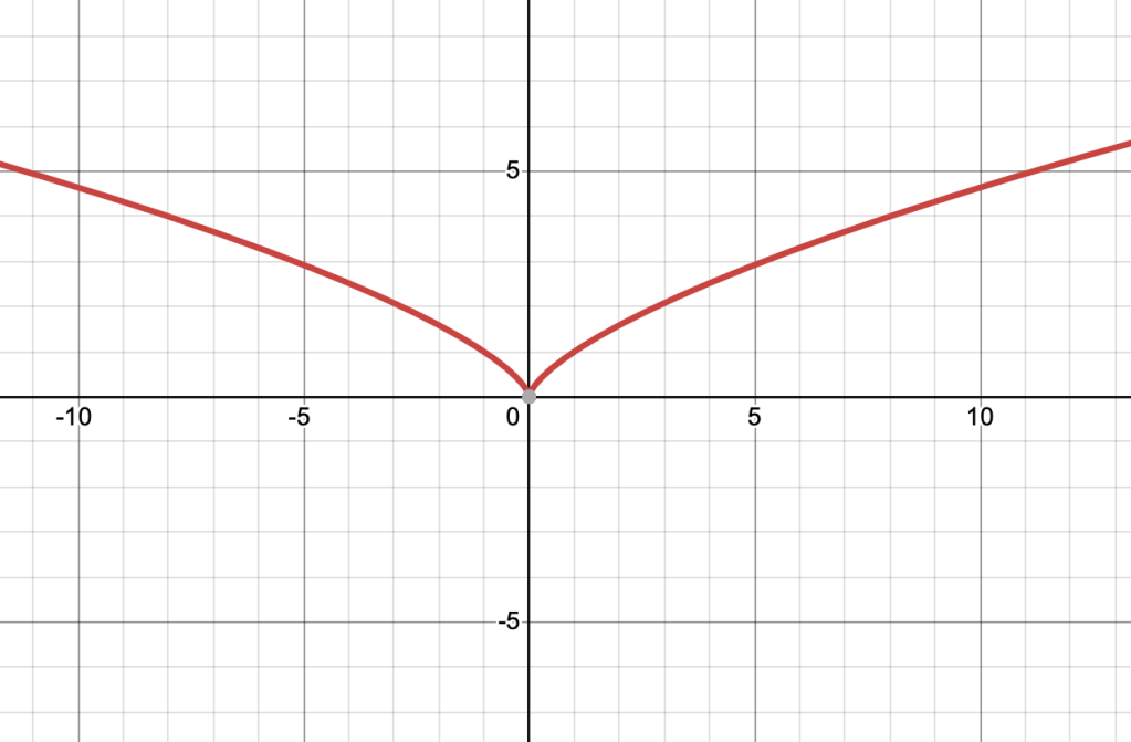
Example: $x^2 = y^3$

Notice that this curve has a cusp at (0, 0).

To find the lift of this curve in $\mathbb{R}^2 \times \mathbb{RP}^1$ , we must obtain the value of the slope of the tangent line to the curve at each point. We can easily do so by describing this curve as the path of a particle (i.e. parameterizing the curve) and finding the velocity of the particle at each point.

$x^2 = y^3$ can be parameterized by $t \mapsto (x(t), y(t)) = (t^3, t^2)$ .

The velocity vector at the corresponding point is given by $(\dot{x}(t), \dot{y}(t)) = (3t^2, 2t)$ .

Since we are working with the projectivization of the tangent space, we are interested in the space of lines passing through the origin of the tangent space. The velocity vector in the projectivization of the tangent space becomes $[3t^2, 2t]$ . For $t \neq 0$ , this is just $[3t, 2]$

Notice that when $t = 0$ , the corresponding point on the curve is $(0, 0)$ , the cusp.

As $t \rightarrow 0$ , $[3t, 2] \rightarrow [0, 2] = [0, 1]$ . Hence, the lifted curve $\tilde{\mathcal{C}}$ has a limit as $t \rightarrow 0$ ; it is $(0, 0, [0, 1])$ . But is it smooth at $t = 0$ ?

In a neighbourhood of $[0, 1]$ , the 2nd component is non-zero. We look at the parameterization of the p-value on the chart $[x, y] \mapsto \frac{x}{y}$ . This would be given by $t \mapsto [3t^2, 2t] \mapsto [\frac{3}{2}t, 1] \mapsto \frac{3}{2}t$ , which is obviously smooth.

Thus, the lifted curve $\tilde{\mathcal{C}}$ is smooth in $\mathbb{R}^2 \times \mathbb{RP}^1$ .

Resolving the singularity of $x^2 = y^3$ by blowing-up the plane at (0,0)

Key: When we blow-up the plane at (0, 0), we are really considering a new geometric object. It lives inside $\mathbb{R}^2 \times \mathbb{RP}^1$ , given by:

$\tilde{\mathbb{R}^2} = \{ ((x, y), [u, v]) \in \mathbb{R}^2 \times \mathbb{RP}^1 : xv = yu \}$

A point in our new space is the point in the original space + the line passing through that point and the origin

At the original origin, we now have instead a space of lines; we have replaced (0, 0) with a copy of $\mathbb{RP}^1$ .

When we consider $x^2 = y^3$ in $\tilde{\mathbb{R}^2}$ , we see each point on the curve as not only that point, but also the line connecting that point to the origin.

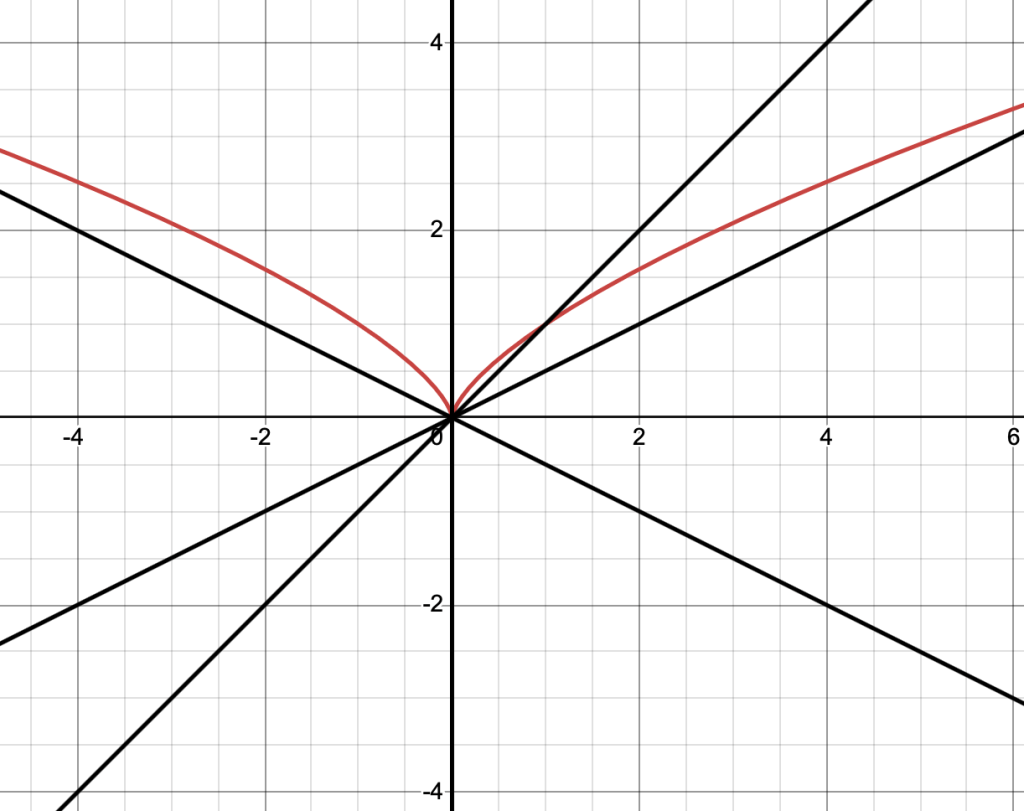
Tracing the curve with the space of lines at (0, 0).

Algebraically, this would be given by:

Let $x = ty$ (Why not $y = tx$ ? This is because the slope of each line tracing the curve given by $\frac{x}{y}$ is always finite, but $\frac{y}{x}$ is not.)

Then, the equation becomes:

$(ty)^2 = y^3$

$\Rightarrow y^2(t^2 - y) = 0$

$\Rightarrow y^2 = 0, y = t^2$ .

These two curves we obtain live in $\tilde{\mathcal{R}^2}$ .

Notice the difference between the lifting of $\mathcal{C}$ to $\tilde{\mathcal{C}}$ and the blowing up of $\mathcal{C}$ at its singularity. We are dealing with 2 different spaces. In the first method, we embed $\mathcal{C}$ in $\mathbb{R}^2 \times \mathbb{RP}^1$ ; $\mathcal{C}$ is the projection of $\tilde{\mathcal{C}}$ along the p-axis. In the latter method, we are embedding $\mathcal{C}$ in $\tilde{\mathcal{R}^2}$ .

Lifting to a Legendrian Curve v.s. Blowing Up at a Point

Share this:

Leave a Reply Cancel reply