Arnold’s PDE: Constructing Isotropic Manifolds & the Euler Equation Example (Updated: 17/10/2025)

This post is based upon my reading of part of the 2nd chapter of Arnold’s PDE. The goal is to locally construct the 1-graphs of solution to the Cauchy problem.

Recall, the Cauchy problem is the following: given a smooth hyper surface of dimension n-1, $\Gamma^{n-1}$ in x-space and an initial function $u_0$ defined on $\Gamma^{n-1}$ . Then, for a first-order PDE $F(x, u, p) = 0$ , find a solution $u$ such that $u|_{\Gamma^{n-1}} = u_0$ .

Step 1: How do we extend $\Gamma^{n-1}$ to be an (n-1)-dimensional isotropic initial sub-manifold of the 2n-dimensional manifold given by $F(x, u, p) = 0$ ?

(Rationale behind this step: Once we have such an (n-1)-dimensional sub-manifold, we can construct the local 1-graph of a solution by drawing the set of all characteristic curves passing through a neighborhood of a non-characteristic point on the sub-manifold.)

In a small neighborhood of $q \in \Gamma^{n-1}$ , we can (after smooth change of coordinates) assume that $\Gamma^{n-1}$ is given by $f(x_1, ..., x_{n-1}) = 0$ and $x_n$ is orthogonal to $\Gamma^{n-1}$ at $q$ . Thus, the derivatives along the directions tangent to $q$ are given by $\frac{\partial f}{\partial x_1}, ..., \frac{\partial f}{\partial x_{n-1}}$ . Thus, in a small neighborhood, the $p_1, ..., p_{n-1}$ coordinates of the (n-1)-dimensional isotropic sub manifold are given by: $p_1 = \frac{\partial f}{\partial x_1}, ..., p_{n-1} = \frac{\partial f}{\partial x_{n-1}}$ .

What about the $p_n$ coordinate? i.e. how do we find the derivative of the direction orthogonal to $\Gamma^{n-1}$ at $q$ ? By our choice of coordinates, a unit vector in this direction is given by $v = (0, 0, ..., 0, 1)$ .

Recall: the characteristic vector field of $F(x, u, p) = 0$ is given by $\dot{x} = F_p$ , $\dot{y} = pF_p$ , and $\dot{p} = -(F_x + pF_y)$ . The projection of the vector onto the x-space at $q$ is just the x-component of the vector, i.e. $\dot{x} = F_p$ .

If $F_p$ is not tangent to $\Gamma^{n-1}$ at $q$ , then $F_p \cdot v = 0$ . Recall from above, $v = (0, 0, ..., 0, 1)$ . Since $F_p = (\frac{F}{\partial p_1}, ..., \frac{F}{\partial p_n})$ , this means $\frac{F}{\partial p_n} \neq$ . By the implicit function theorem, we can locally express $p_n$ as a function of $x_1, ..., x_n, u, p_1, ..., p_{n-1}$ , say $p_n = h(x_1, .., x_n, u, p_1, ..., p_{n-1})$ , so that $F(x_1, ..., x_n, u, p_1, ..., p_{n-1}, h(x_1, ..., p_{n-1}) = 0$ .

Step 2: Constructing an isotropic sub-manifold of dimension $\Gamma^n$ containing $\Gamma^{n-1}$ .

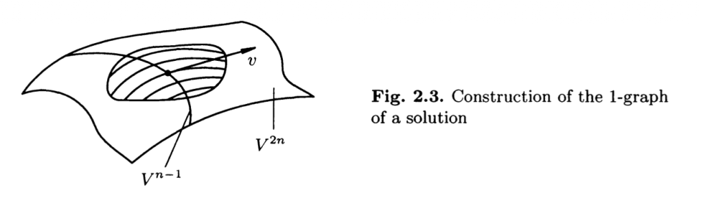
Given a neighbourhood of a point $\Gamma^{n-1} \subset V^{2n}$ that is not tangent tangent to the characteristic vectors, draw the set of all characteristics passing through the points in this neighbourhood. We obtain a n-dimensional sub-manifold $\Gamma^n$ .

Claim: $\Gamma^n$ is isotropic.

In this figure, $\Gamma^{n-1} := V^{n-1}$ is a 1-dimensional curve. We draw the set of characteristic curves passing through $\Gamma^{n-1}$ . Notice that for each $z \in V^{n-1} \cap \Gamma^n$ , by construction, $T_z \Gamma^n$ is isotropic.

In this figure, $\Gamma^{n-1} := V^{n-1}$ is a 1-dimensional curve. We draw the set of characteristic curves passing through $\Gamma^{n-1}$ . Notice that for each $z \in V^{n-1} \cap \Gamma^n$ , by construction, $T_z \Gamma^n$ is isotropic.

Important geometric observation: $\Gamma^n$ ‘flow’ of the initial isotropic sub-manifold along the characteristic curves, i.e. we obtain this sub manifold by translating $\Gamma^{n-1}$ along the characteristics.

By our assumption $\Gamma^{n-1}$ is isotropic, and so $d \alpha|_{T_z \Gamma^{n-1}} = 0$ .

Claim: $d\alpha |_{\Gamma^n} = 0$ i.e. $\Gamma^n$ is isotropic.

Let $v$ be the characteristic vector field.

Homotopy formula (I’m taking it for granted, for now):

$L_v \alpha (\xi) = d\alpha(v, \xi) + d(\alpha(v))(\xi)$ , where $\xi \in T \Gamma^n$ .

The characteristic vector is the skew-orthogonal complement of $V^{2n} \cap K^{2n}$ , and so for any $\xi \in T\Gamma^n \subset T V^{2n}$ , $d\alpha(v, \xi) = 0$ .

Since $v$ is also in the contact plane, $\alpha(v) = 0$ .

And so, $L_v \alpha = 0$ .

This means that the phase flow of the characteristic field maps the form into itself, i.e. for any $\xi \in T_z \Gamma^n$ , we have:

$\alpha(\xi) = \alpha(d\phi^t(\xi))$ where $d\phi^t$ is the corresponding linear map between the tangent spaces of the phase flow $\phi^t: z \mapsto \phi^t(z)$ .

Since $d\phi^t$ is a bijection, it follows that for any $\zeta \in T_{\phi^t(z)} \Gamma^n$ , there exists $\xi \in T_z \Gamma^n$ such that

$d\phi^t(\xi) = \zeta$ .

Key: Any point on $\Gamma^n$ lies on a unique characteristic curve (aka phase curve), i.e. for any point on $\tilde{z} \in \Gamma^n$ , there exists $z \in \Gamma^{n-1}$ such that $\phi^t(z) = \tilde{z}$ for some phase flow $\phi$ and for some time $t$ . Thus, the action of $\alpha$ on $T_{\tilde{z}} \Gamma^n$ is the ‘same’ as the action of $\alpha$ on $T_z \Gamma^n$ . But since for $z \in \Gamma^{n-1}$ , $T_z \Gamma^n= \text{span} \{ T_z \Gamma^{n-1}, v \}$ , $\alpha |_{T_z \Gamma^n} = 0$ . Hence, $\alpha |_{T_{\tilde{z}} \Gamma^n} = 0$ . Since $\tilde{z} \in \Gamma^n$ is arbitrary, it follows that $\alpha|_{\Gamma^n} = 0$ .

$d\alpha$ is also mapped into itself by the field $v$ (not sure how this is obtained, perhaps we can use the homotopy formula for 2-forms; still thinking about it).

Also, why do we need to show $\Gamma^n$ is isotropic?

It follows that $\Gamma^n$ is an integral sub manifold of the contact structure and is also a sub manifold of the equation.

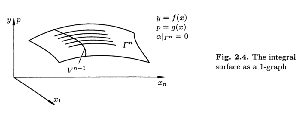
Step 3: if $\Gamma^n$ can be locally projected in a one-to-one manner onto the x-space, it is locally a 1-graph of a solution to the PDE.

Key: the one-to-one projection means locally, the $y, p$ variables can be written as differentiable functions of $x$ , i.e. $y = f(x), p = g(x)$ .

Since $\Gamma^n$ is an integral manifold of the contact structure, i.e. $latex \alpha|_{\Gamma^n} , and so it follows that

$dy - pdx = 0$

Since $y = f(x)$ , $dy = \sum_{k=1}^n \frac{\partial f}{\partial x_i} dx_i$ , and the above equation becomes:

$sum_{k=1}^n \frac{\partial f}{\partial x_k} dx_k - \sum_{k=1}^n g_k dx_k = 0$

This means that $g_k = \frac{\partial f}{\partial x_k}$ , which means that $\Gamma^n$ is a 1-graph.

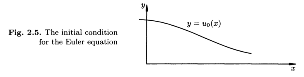
Example: Cauchy problem for Euler equation $u_t + u u_x = 0$ with the initial curve $t = 0$ and initial function $y = u_0(x)$ .

I will clarify in advance my use of variables. Here, the time for the phase flows will be denoted using $\tau$ . The (t, x)-plane is the x-space, and the (t, x, y)-space is the space of 0-jets.

This is the graph of the initial function when we restrict the space to the (x, y)-plane.

The characteristic vector field projected into the space of 0-jets is given by $\dot{t} = 1, \dot{y} = 0, \dot{x} = y$ . Notice that for a quasi-linear equation, everything can be considered in the space of 0-jets. We can simply forget about the p-value. Why is it that we can simply forget about the p? Why does setting $\dot{y} = 0$ not affect anything?

Answer: This is because the x and y-components of the characteristic vector are given by $\dot{x} = F_p$ and $\dot{y} = pF_p$ . Since the PDE is given by $F(x, y, p) = a_1(x, y)p_{x_1} + ... + a_n(x, y)p_{x_n} + f(x, y) = 0$ , it follows that $F_p$ is independent of $p$ and $pF_p = -f(x, y)$ , which is also independent of $p$ .

Recall: $\Gamma^n$ is the family of curves obtained by translating the initial sub manifold $\Gamma^{n-1}$ along the characteristics. And because of the ‘nice’ projection where we can forget about the p-value, the 0-graph is the family of curves obtained by translating the initial graph $y = u_0(x)$ along the characteristics in the (t, x, y)-space.

The characteristics in the (t, x, y)-space are the phase curves of:

$\dot{t} = 1$

$\dot{y} = 0$

$\dot{x} = y$

Let $\tau$ be the time, then the phase curves are given by $\phi(\tau) = (\tau + t_0, y_0 \tau + x_0, y_0)$ .

The initial curve and function gives us a set of $(t_0, x_0, y_0) = (0, x_0, u(x_0))$ . Hence, the corresponding phase curves are $\phi(\tau)_{x_0} = (\tau, u(x_0) \tau + x_0, u(x_0))$ .

Let’s look at the example when $u(x) = x^2$ . Then, for a fixed $\tau$ , the translated initial curve is parameterized by:

$t = \tau$

$x(s) = \tau s^2 + s$

$y(s) = s^2$ ,

where $s$ is the x-value input on the initial $u(x) = x^2$ curve.

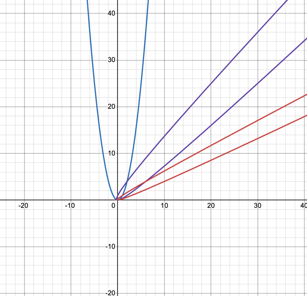
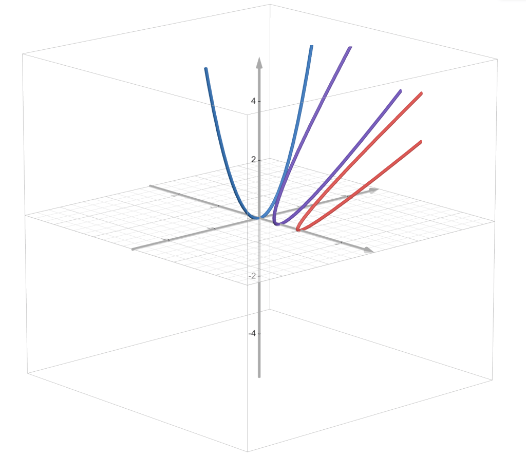
The projection of these translated curves for different time onto the (x,y)-plane is:

The blue curve is when $\tau = 0$ , the purple curve is when $\tau = 1$ , and the red curve is when $\tau = 2$ .

The blue curve is when $\tau = 0$ , the purple curve is when $\tau = 1$ , and the red curve is when $\tau = 2$ .

In the (t, x, y)-space, this is given by:

Interesting: the surface that we construct might have a curve of critical values under the projection $\pi: (x, y, p) \mapsto (x, y)$ .

Let’s look at the most simple example where the initial curve is $t = 0$ and the initial function is given by $u_0(x) = x$ .

The phase curves are described by:

$t(\tau) = \tau + t_0$

$x(\tau) = u_0(x_0)\tau + x_0$

$y(\tau) = u_0(x_0)$

which in this case simplify to:

$t(\tau) = \tau$

$x(\tau) = x_0 \tau + x_0$

$y(\tau) = x_0$

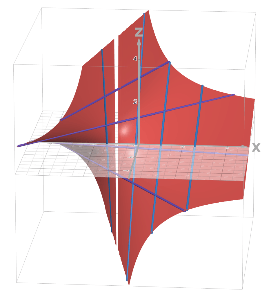
The surface, i.e. the 0-graph, is the set of all translated initial curves along the phase curves. We can also see it as the image of the map:

$\Psi: (x_0, \tau) \mapsto (\tau, x_0\tau + x_0, x_0) =: (t, x, y)$

Notice that the image can also be described as the graph of $y = \frac{x}{t+1}$ .

The red surface is the graph of $y = \frac{x}{t+1}$ . The purple lines lying on the surface are the phase curves. The blue lines lying on the surface are the translated initial curves along the phase curves.

The critical curve of this surface is the intersection between the plane $t = -1$ and the surface. The projection of this curve onto the (t, x)-plane is the point (-1, 0).

Arnold’s PDE: Constructing Isotropic Manifolds & the Euler Equation Example (Updated: 17/10/2025)

Share this:

Leave a Reply Cancel reply