Understanding Contact Structure Through Legendrian Curves: A Comparison Between Thurston’s Approach and Arnold’s Approach

I have been working through the section on contact structures in Arnold’s PDE for a while now, and my understanding of it has been shaky at best. So, it only made sense to look at Thurston’s approach when I found out that his book also had a section on contact structure. The two of them have very different approaches to looking at this concept. I will try to justify what I am about to claim below throughout this post:

The notion of contact structure is really just an extension of the fundamental theorem of calculus. In his PDE book, Arnold gave us the ‘differentiation’ approach to understanding contact structure; in his 3D Geometry and Topology book, Thurston gave us the ‘integration’ approach to understanding it.

Arnold introduced contact structure through the space of 1-jets. The contact structure is the plane field that naturally arise when we consider the set of tangent vectors at each point $(x, y, p)$ such that $\frac{dx}{dy} = p$ . I find that this approach is very concrete; the contact structure is not simply a concept that came out of thin air, rather it is a generalization of this very geometric and intuitive structure that really requires only the most simple calculus concepts to understand. But somehow (and this is probably the fault of my own limited imagination), this made me conform to only thinking about this structure through the lens of ‘differentiating’. For me, the crux of contact structures (the standard one, to be specific) was the value of p, which was the derivative of some kind of curves.

To be honest, this realization only occurred to me after solving one of the exercises in Thurston’s book and seeing the difference between my train of thought and that of which Thurston wrote in the book (I will mention this below).

Thurston introduced contact structures as a kind of plane fields that is as non-integrable as possible. I really like this sentence he wrote:

We will take some time to develop the basic picture for contact structures, because they give an interesting example of a widely occurring pattern for manifolds that is hard to see until your mind and eyes have been attuned.

The first time that I read it, I was quite surprised. I naively thought to myself: “But aren’t the integral manifolds of the contact structures just the 1-graph of some solution to a PDE? Why is that so difficult to see?”

Yup, they sure are.

BUT I did not realize how not easy it was for me to think about things backward. Like I said before, I got into the habit of first dealing with the PDE, constructing a vector field using the contact structure and the PDE, and then obtaining the manifold.

The first contact structure Thurston gave in the book is the $\tau$ plane field such that the plane at each point $(x, y, z) \in \mathbb{R}^3$ is spanned by the vectors $(1, 0, 0)$ and $(0, 1, x)$ . And (again, this is one of those sentences that just speaks for itself):

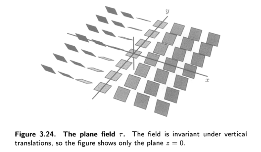
To understand $\tau$ , it helps to think about Legendrian curves, which are curves in $\mathbb{R}^3$ whose tangent vectors are always contained in $\tau$ .

So yes, directly looking at the contact structure tells us nothing about it; we must know how we can move in this space of plane field. Essentially, the Legendrian curves are the possible paths of moving inside a contact structure.

Exercise 3.7.1 (Legendrian lifts). Given a piecewise differentiable curve $\gamma: [0, 1] \mapsto \mathbb{R}^2$ in the xy-plane, and a point in $\mathbb{R}^3$ that projects to $\gamma(0)$ , there is a unique lift of $\gamma$ to a Legendrian curve $\tilde{\gamma}: [0, 1] \rightarrow \mathbb{R}^3$ that projects to $\gamma$ .

My first reaction had been:

The plane field is described by $0 = - xdy + dz$ , and so, the planes are the set of tangent vectors satisfying $\frac{dz}{dy} = x$ at each point. This means that the curve $\gamma(t)$ gives us the value of $\phi'(z)$ at each point. To find $\tilde{\gamma}$ , it suffices to find $z \mapsto \phi(z)$ . The initial point $p = (\phi'(z_0), \phi(z_0), z_0) \in \mathbb{R}^3$ is the initial value.

Let’s see how this is actually done through an example. Turns out, I did not have to find the actual $z \mapsto \phi(z)$ .

Suppose we are given the curve:

$\gamma: [0, 2\pi] \rightarrow \mathbb{R}^2$

$\gamma: t \mapsto (cos(t), sin(t))$

and the initial value $(cos(0), sin(0), 0)$ .

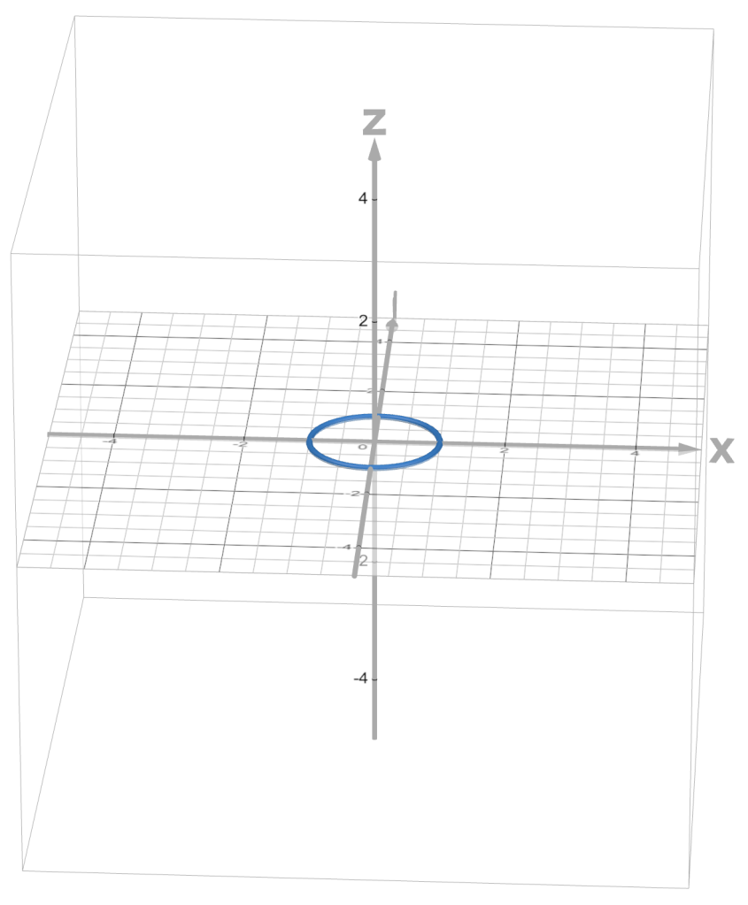
We know that $\tilde{\gamma}(t) = (cos(t), sin(t), z(t))$ . Our goal is to find $z(t)$ .

Key: $\tilde{\gamma}$ is the 1-graph of $z \mapsto \phi(z)$ . And so, by definition:

$\frac{\frac{d z(\tau)}{d\tau}|_{\tau = t}}{\frac{d sin(\tau)}{d\tau}|_{\tau = t}} = cos(t)$ .

Hence, it follows that:

$\frac{d z(\tau)}{d\tau}|_{\tau = t} = \frac{d sin(\tau)}{d\tau}|_{\tau = t} \cdot cos(t)$

$\Rightarrow \dot{z} = cos^2(t)$

$\Rightarrow z(t) = \frac{t}{2} + \frac{sin(2t)}{4} - z(0) = \frac{t}{2} + \frac{sin(2t)}{4}$

Thus, the Legendrian lift that we obtain is:

$\tilde{\gamma}: t \mapsto (cos(t), sin(t), \frac{t}{2} + \frac{sin(2t)}{4})$

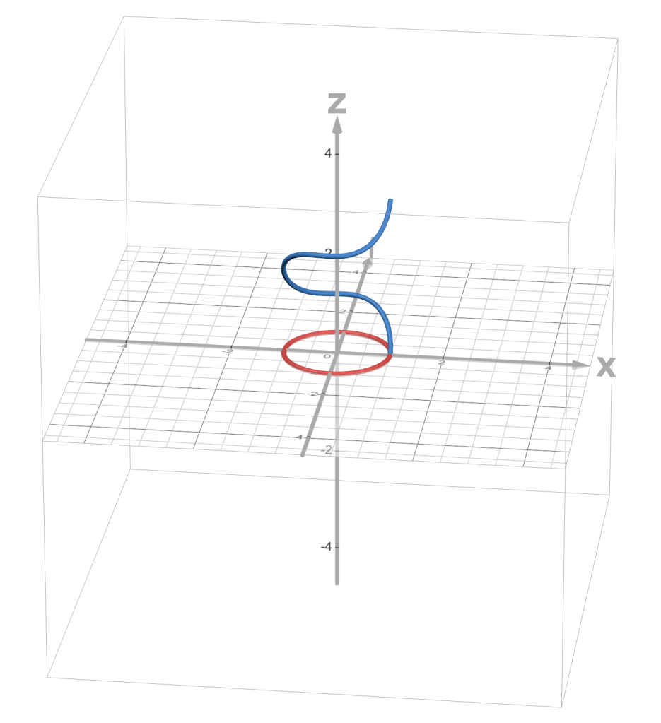
The end point of this Legendrian curve is $(cos(2 \pi), sin(2 \pi), \pi)$ . The height difference between the end point and the starting point is $\pi$ . Notice that the area enclosed by our $\gamma$ curve is also $\pi$ . Is this a coincidence?