Exploring the Lorentzian Space: Sphere of Radius √-1

This post is based upon my reading of section 2.3 of Chapter 2 of Thurston’s Three Dimensional Geometry and Topology. In particular, we will be looking at the analogue to the unit sphere (in Euclidean space $\vb{E}^n$ ) in Lorentzian space $\vb{E}^{n, 1}$ .

The Lorentzian space $\vb{E}^{n, 1}$ is $\mathbb{R}^{n+1}$ endowed with metric $\eta = - dx_0^2 + dx_1^2 + ... + dx_n^2$ . This metric is associated with the quadratic form: $Q^{-}(x) = -x_0^2 + x_1^2 + ... + x_n^2$ .

The $x_0$ direction represents time and the subspace spanned by $\{ x_1, ..., x_n \}$ represents space (when n=3, this gives us the model for special relativity).

A vector $x$ is space-like if $Q^{-}(x)$ is positive, time-like if $Q^{-}(x)$ is negative, and light-like if it is zero. The length of a vector is given by $\sqrt{Q^{-}(x)}$ (analogous to the Euclidean case). Hence, time-like vectors have imaginary length.

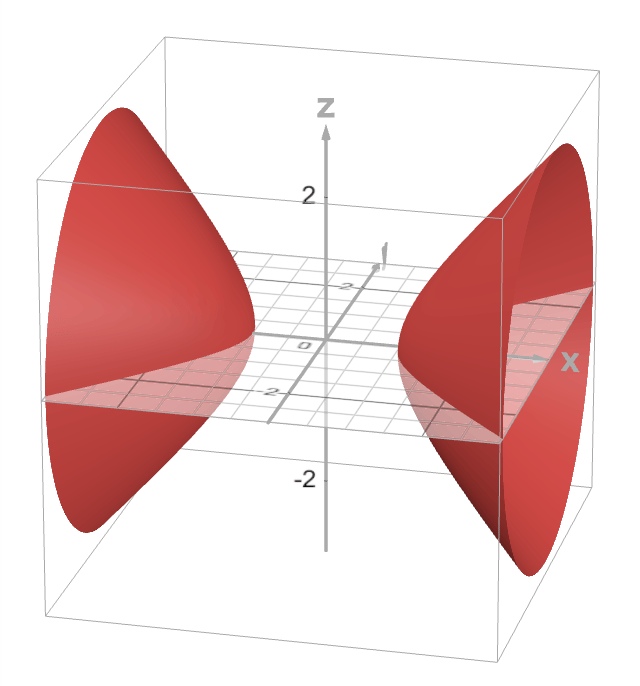
In this post, we will study the sphere of radius $I$ about the origin in $\vb{E}^{n,1}$ , i.e. the set of ‘unit length’ time-like vectors. This set is (let’s call it $\vb{H}$ ) in fact, a hyperboloid. In $\mathbb{R}^{2,1}$ , it looks like:

Claim: the restriction of the metric $\vb{H}$ gives us a positive definite Riemannian metric.

Approach 1: we compute the metric on this surface.

Key: to make computations more simple, notice that $\vb{H}$ can be seen as the graph of a function over the $x_0 = 0$ hyperplane.

Define $\Psi: \mathbb{R}^n \rightarrow \vb{H} \subset \mathbb{R}^{n+1}$ given by

$\Psi(y_0, ..., y_n) = (x_0, x_1, ..., x_n)$ with

$x_0 = \sqrt{1+||y||^2}$

and $x_k = y_k$ for any $k \geq 1$ .

This gives us one component of the hyperboloid $\vb{H}$ . We can similarly derive the metric on the other component, and show that it will be the same.

Notice that $\Psi^{-1}$ on this component of $\vb{H}$ gives us a chart.

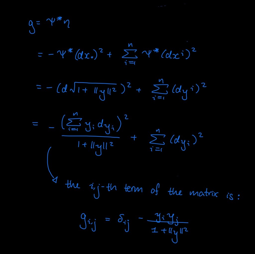
I will attach a screenshot of my computations below (I am too lazy to Latex everything out):

This is the metric matrix with respect to the basis $dy_1, ..., dy_n$ . To show that this matrix is indeed positive definite, it suffices to compute its eigenvalues.

It is not difficult to spot the eigenvectors.

Given a point $(y_1, ..., y_n) \in \mathbb{R}^n$ , notice that:

$g(y) = y \cdot \frac{1}{1 + ||y||^2}$

and for any $w \perp y$ , $g(w) = w$ .

Approach 2: Thurston said in his book that the reason we have a positive definite Riemannian metric on $\vb{H}$ is because the tangent vector to $\vb{H}$ has real length. Is this sufficient? I am still very new to the notion of putting metrics on sub manifolds. He was saying the restriction of $\eta$ to $\vb{H}$ . Is there a difference between the restriction of a metric in the ambient space to a manifold and the induced metric?

Interesting: A subset of $\mathbb{RP}^n$ on $\vb{H}$

On the sphere, we can construct $\mathbb{RP}^n$ by identifying antipodal points. Again, we can get a subset of $\mathbb{RP}^n$ by identifying antipodal points of $\vb{H}$ . But since $\vb{H}$ consists of 2 disjoint components, this subset can be simply described by one component. Thurston called this the hyperboloid model of hyperbolic space.

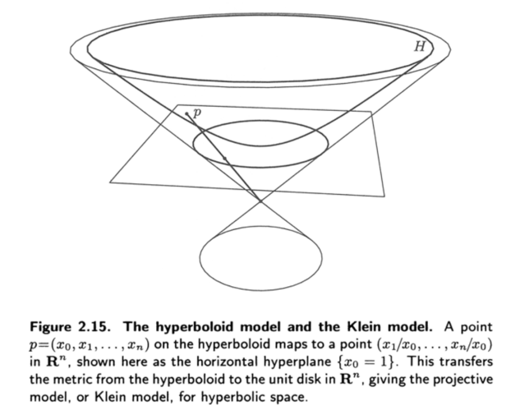
We can also describe the same subset by mapping $\vb{H}$ onto the unit disk by the lines $(t, x_1 t, ..., x_n t)$ passing through the origin. Please see the following excellent figure that Thurston had put in his book:

This gives us the Klein model of hyperbolic space.

Thinking about: the metric on the Klein disk is not the induced metric, but the push-forward of the hyperboloid’s metric by central projection. (As you can probably tell, I have now become quite confused with the various ways which we can define new metrics…, still in the process of figuring everything out.)

Orthogonal Complement: this is analogous to the Euclidean space. Given a non-zero vector x, its orthogonal complement $x^{\perp}$ is n-dimensional.

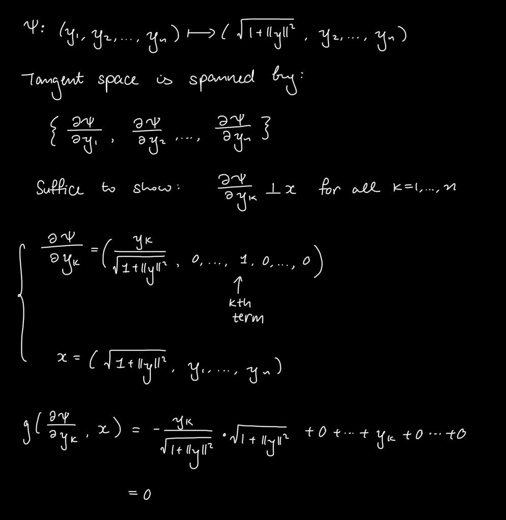
Claim: for any point $x \in \vb{H}$ , $T_x \vb{H} = \{ y \in \vb{E}^{n, 1}: y \perp x \}$ .

Proof (I have again attached a screenshot of my work because I am feeling exceedingly lazy):

Isometries of $\vb H$

Analogous to the Euclidean space where the isometries of the sphere are exactly the orthogonal transformations of the Euclidean space, in the Lorentzian space, the isometries of $\vb{H}$ are exactly the orthogonal transformations of the Lorentzian space. The orthogonal transformations are the linear transformations of $\mathbb{R}^{n+1}$ preserving the quadratic form $Q^{-}(x) = -x_0^2 + x_1^2 + ... + x_n^2$ .

Since $\vb{H}$ is the zero-set of $Q^{-}$ , any non-trivial orthogonal transformation of $\vb{E}^{n, 1}$ , $O(n, 1)$ induces a non-trivial isometry on $H$ . So it now remains to show all isometries of $\vb{H}$ are indeed elements of $O(n, 1)$ . It suffices to show that O(n, 1) acts transitively and isotropically on H. Recall: a group acts isotropically on $\vb{H}$ if at any point $p \in H$ and any isometry, $B$ , in the tangent space $T_p \vb{H}$ , there exists a group element $A \in O(n, 1)$ fixing $p$ such that $dA|_p$ coincides with $B$ .

Currently thinking about: how do these 2 statements imply that $O(n, 1)$ is the group of isometries for $H$ ?

Transitivity

Key: use reflection across the orthogonal complement of $v := p - q$ .

Notice that $g(p-q, p-q) = g(p, p) + g(p, -q) + g(-q, p) + g(-q, -q) = -2(1 + g(p, q))$ is non-zero for $p \neq q$ (where $g$ is the Lorentzian inner product).

Hence, we can define the Lorentzian reflection across $v$ :

$R_v(x) = x - 2\frac{g(x, v)}{g(v, v)}v$

When $x \in v^{\perp}$ , $R_v(x) = x$ .

$R_v(p) = p - 2 \frac{g(p, p-q)}{g(p-q, p-q)}(p-q)$

$= p - 2\frac{-1 - g(p, q)}{-2(1 + g(p, q)}v$

$= p - v$

$= q$

Similarly, we can show that $R_v(q) = p$ .

It is not difficult to check that $R_v$ is an element of $O(n, 1)$ .

Isotropicity

From part a), it suffices to consider $p = (1, 0, ..., 0)$ .

From the previous exercise, $T_p \vb{H}$ = $p^{\perp}$ (this is the n-dimensional space-like subspace of $E^{n, 1}$ ). The Lorentzian metric when restricted to this subspace is positive definite. Thus, we can find an orthonormal basis in $p^{\perp}$ such that we have the usual Euclidean space of dimension n. Let $B$ be an isometry of this tangent space; then $B$ is a Euclidean isometry and it fixes the origin. We can show that $B$ is an orthogonal transformation on $\mathbb{R}^n$ , i.e. $B^{T}B = I$ .

We now extend $B$ to a linear map $A$ on $\mathbb{R}^{n+1}$ .

Let $A = \begin{bmatrix} 1 & 0_{1 \times n} \\ 0_{n \times 1} & B \end{bmatrix}$ .

It is easy to see that $A(p) = p$ and

$A^{T} \eta A = \begin{\bmatrix} 1 & 0_{1 \times n} \\ 0_{n \times 1} & B^{T} \end{bmatrix} \begin{\bmatrix} -1 & 0_{1 \times n} \\ 0_{n \times 1} & I_n \end{\bmatrix} \begin{\bmatrix} 1 & 0_{1 \times n} \\ 0_{n \times 1} & B \end{bmatrix}$

$= \begin{\bmatrix} -1 & 0_{1 \times n} \\ 0_{n \times 1} & I_n \end{\bmatrix}$

Thus $A \in O(n, 1)$ .

Exploring the Lorentzian Space: Sphere of Radius √-1

Share this:

Leave a Reply Cancel reply