Differentiation of Vector Fields on Manifolds (Arnold’s Math. Methods & Penrose’s The Road to Reality)

Part 1: We will look at the geometric meaning behind differentiating vector fields in the Euclidean space using the Poisson brackets. This is based upon my reading of the section on Lie algebra in Arnold’s Mathematical Methods of Classical Mechanics.

Part 2: By considering the tangent bundle corresponding to a smooth manifold M, we can define vector fields on M. Is it possible for us to do something similar in the Euclidean space, i.e. can we ‘differentiate’ vector fields? How do we even define differentiation when the coordinates for each patch may be completely different? This is based upon my reading of chapter 14 of Penrose’s The Road to Reality.

Part 1:

Let M be a smooth manifold and A a smooth vector field on M. There are 2 geometric objects that are correspond uniquely to A:

1) one-parameter group of diffeomorphisms (or flows), i.e. for fixed $t \in \mathbb{R}$ , we have

$A^t : M \rightarrow M$ such that

$\frac{d}{dt}|_{t=0}A^t x = A(x)$ (where $A(x)$ is the vector of A defined at x.

2) first-order differential operator $L_A$ , i.e. differentiating functions in the direction of $A$ . Given $\rho : M \rightarrow \mathbb{R}$ ,

$(L_A \rho)(x) = \frac{d}{dt}|_{t=0} \rho(A^t x)$

The geometry behind the Poisson bracket arises from the very simple question: given 2 vector fields A, B on M and an initial point $p \in M$ , do we reach the same destination by first traveling along A then B or first traveling along B then A? i.e. for fixed $s, t \in \mathbb{R}$ , do we have:

$A^s B^t (p) = B^t A^s (p)$ ?

No! Consider $A = \frac{\partial}{\partial x_2}$ and $B = x_2 \frac{\partial}{\partial x_1} - x_1 \frac{\partial}{\partial x_2}$ on $\mathbb{R}^2$ . Choose $p$ to be the origin. Then, we have:

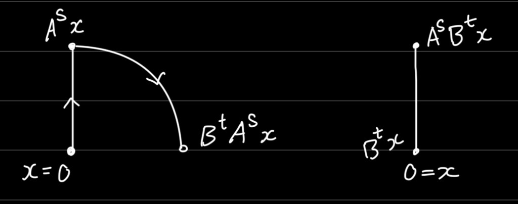
The Poisson bracket gives us a way to measure the amount of non commutativity of two vector fields (and their corresponding flows). How do we measure such thing? Perhaps we look at how ‘far’ how the two points $B^t A^s x$ and $A^s B^t x$ are from each other? We can do that. In fact, we can assess this difference by looking at the difference in the values of a function at those two points. Let’s see what that means:

Let $\Delta(t; s; x) = \phi(A^s B^t x) - \phi(B^t A^s x)$ .

Notice: when $s = 0$ or $t = 0$ , $\Delta(t; s; x) = 0$ . Hence, the Taylor expansion looks like: $\Delta(t; s; x) = t s h(t; s; x)$ .

The Poisson bracket is the principal bilinear term of $\Delta(t; s; x)$ .

Lemma: $\frac{\partial^2}{\partial s \partial t}|_{s=t=0} (\phi(A^s B^t x) - \phi(B^t A^s x)) = (L_B L_A \phi - L_A L_B \phi)(x)$ .

Proof: $\frac{\partial}{\partial}|_{s=0} \phi(A^s B^t x) = lim_{h \rightarrow 0} \frac{\phi(A^h)(B^t x) - \phi(A^0)(B^t x)}{h} = (L_A \phi)(B^t x)$

(the last equality follows by definition of $L_A$ .)

Define $\Psi := L_A \phi$ , then

$\frac{\partial}{\partial t}|_{t=0} \Psi(B^t x) = (L_B \Psi)(x) = (L_B L_A \phi)(x)$ .

Similarly, we can show that

$\frac{\partial}{\partial s \partial t}|_{s=0, t=0} \phi(B^t A^s x) = (L_A L_B \phi)(x)$ . $\square$

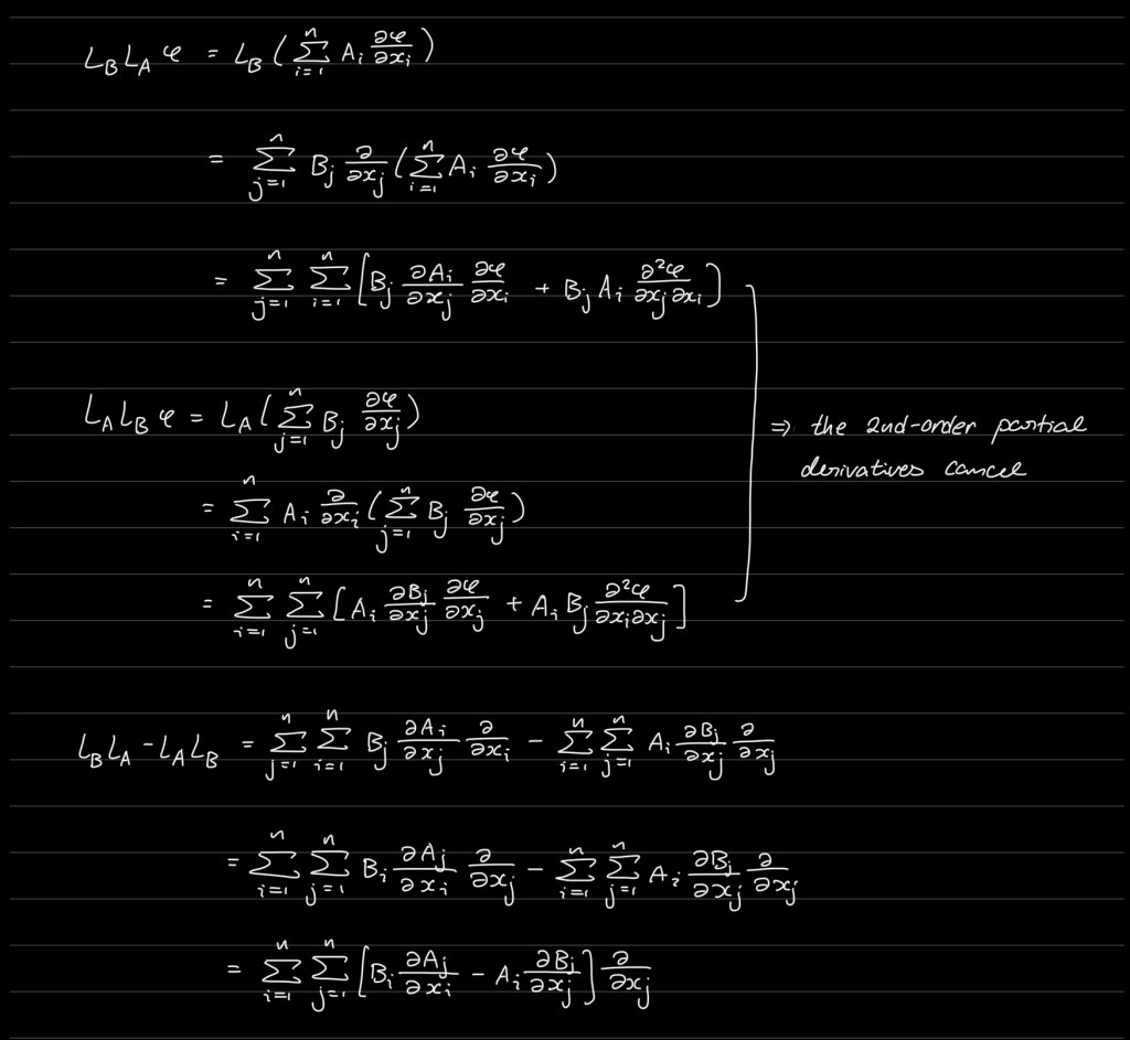
Claim: $L_B L_A - L_A L_B$ is a first-order linear differential operator.

Proof (too lazy to type everything out, so here is a screenshot of my notes):

Condition for commutativity of flows: $A^s B^t = B^t A^s \iff [A, B] = 0$

( $\Rightarrow$ ) this follows by Lemma 1.

( $\Leftarrow$ ) *will follow in an upcoming post.

Let’s look at some examples:

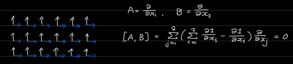
Example of a field that commutes:

Example of a field that does not commute:

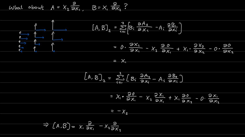
Computing the vector field by computing its flows:

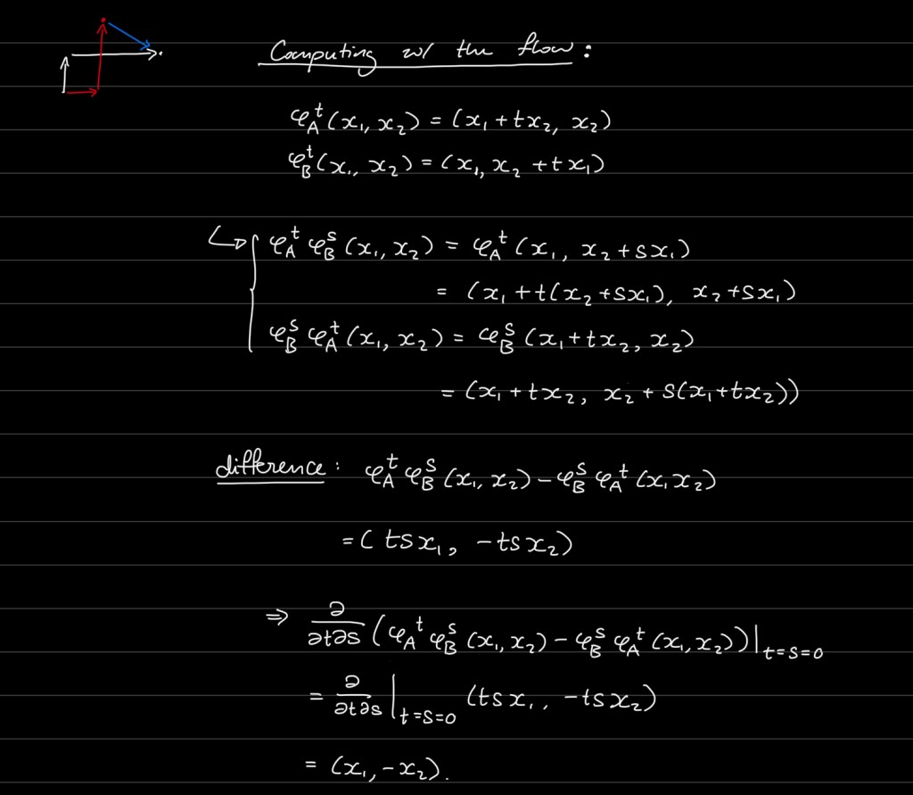
The new flows are hyperbolic curves, $t \mapsto (e^{tx_1}, e^{-tx_2})$ described by the system:

$\dot{x_1} = x_1$

$\dot{x_2} = -x_2$ .

Part 2:

We can represent symmetry groups through their actions on vector spaces; these give us the linear transformations. In terms, for a given symmetry group, the corresponding vector spaces must possess some particular structure which is preserved by these transformations.

Example: the action of the orthogonal group in the Euclidean space preserves the metric structure; this metric structure is what gives us a measure of ‘distance’ between points.

Given a manifold, the notion of local geometry is given by the assignment of local structure to the tangent spaces of the manifold. By assigning a metric structure, we can locally measure the distance between points. By assigning a symplectic structure, we can measure that area of a surface. And on a Riemann surface, we have a notion of ‘angle’ between curves given by the fact that transition maps between charts are conformal. (New understanding: a Riemann surface is one on which we can locally define angles).

Problem: given a general smooth manifold, we do not have a general notion of differentiation. On a small neighborhood, we can assign coordinates $x^1, x^2, ..., x^n$ and differentiate with respect to these coordinates, i.e. $\frac{\partial}{\partial x^1}, ..., \frac{\partial}{\partial x^n}$ . But this is quite meaningless because they depend on the choice of coordinates and answers do not usually match when we pass from on neighborhood to another.

Goal: give a complete notion of ‘derivative’ of geometric objects on a general smooth manifold that is coordinate-independent.

To do so, we need to ask ourselves how we would identify the most simple vector field, a constant field, on a manifold?

In $\mathbb{R}^n$ , this is very easy. Geometrically, it is the field of arrows that are parallel to each other and have the same length. But how do we define parallelism for a general manifold M?

For instance, in hyperbolic geometry, there is no notion of parallelism. Any two lines will intersect at a point.

This means we need to adjust our notion of parallelism.

Let’s look at in detail the geometry of $S^2$ .

Let’s set point p to be the North Pole and $\vec{v}$ to be a vector in the tangent plane of $S^2$ at p.

Which other tangent vectors at other points of $S^2$ are parallel to $\vec{v}$ ?

Let’s first try using the notion of “parallelism” inherited from the embedding in $\mathbb{R}^3$ :

Figure from Penrose’s The Road to Reality

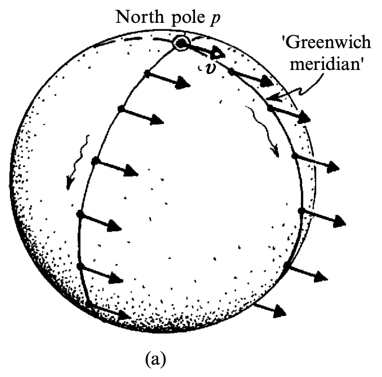
We now run into a problem. Notice that at many points, the vectors parallel to the initial $\vec{v}$ are not actually in the tangent planes, i.e. they are not tangent vectors!

Key: the notion of parallelism on $S^2$ should refer ONLY to the tangent vectors. This idea will probably later be applied to a general manifold M. Parallelism should not refer to the ambient space. What we are going to do is to pull the direction of $\vec{v}$ back into the tangent plane as we gradually move from p to our destination point (the pulling back will be done via projection on to the tangent plane). This definition of parallelism depends on the path we take; when we move differently, the pulling back will be different.

So here is how this is done. Choose a path $\gamma$ from p to q. We divide $\gamma$ into line segments $p_0 p_1, p_1 p_2, ..., p_{N-1} p_N$ ( $p_0, ..., p_N$ are points on $\mathbb{S}^2$ and $p_0 = p$ and $p_N = q$ ). Along each one of the segments, we move $\vec{v}$ parallel to itself (the parallel is inherited from the ambient space $\mathbb{R}^3$ ) and then project onto the tangent space at p. In the limit as $N \rightarrow \infty$ , the answer is well-defined and does not depend on the partition. This is called the parallel transport of $\vec{v}$ along $\gamma$ .

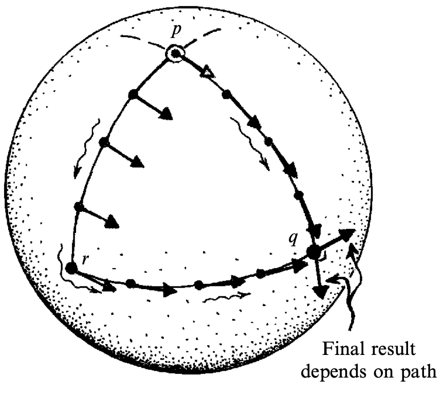
As can be seen in the figure above, parallel transport along different paths give us different results. But what is cool is that the length of the vector is always preserved (this is not true for all types of parallel transport though) and if we are on a unit sphere, the angle between the two vectors is the total area of the loop, i.e. the region surrounded in the negative sense when traveling along the loop in the negative direction.

Now, how can we use this notion of parallel transport to define differentiation of vector fields?

The “difference” arises from the comparison of vectors under parallel transport along some curve $\gamma$ . But since such comparison only makes sense when we are considering infinitesimal displacement from p, we are not interested in one particular curve, rather (as Arnold had said), we are interested in an equivalence class of curves with the same kind of initial ‘velocity’, i.e. the same tangent vector $\omega$ at p.

This gives us a notion of differentiation of vectors. It is called the covariant derivative or connection and is often denoted by $\nabla$ (I find it odd that they would the symbol as they do for the gradient; is there a particular reason?).

Notation: $\nabla_{W}V$ means ‘differentiating’ V along W.

Of course, we have some basic requirements for $\nabla$ to make things nice:

it depends linearly on $W$ (the vector field that is doing the differentiating)
it also satisfies the kind of rules that the differential operator satisfies

Differentiation of Vector Fields on Manifolds (Arnold’s Math. Methods & Penrose’s The Road to Reality)

Share this:

Leave a Reply Cancel reply