Arnold’s Mathematical Methods of Classical Mechanics: Exterior Differentiation

This post is based upon my reading of the section on exterior differentiation in Arnold’s Mathematical Methods of Classical Mechanics.

The exterior of a k-form $\omega$ on a manifold M is a (k+1)-form $d\omega$ on M.

Finding $d\omega$ is analogous to finding the differential of a function or the divergence of a vector field. Let’s see why.

Geometric definition of the divergence of a vector field at a point:

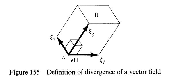
Let A be a vector field on the oriented $\mathbb{R}^3$ , and S be the boundary of the parallelepiped $\Pi$ with edges $\xi_1, \xi_2, \xi_3$ at vertex x.

The flux of A through S is:

$F(\Pi) = \int_S (A, d\hat{n})$

Figure taken from Arnold’s Mathematical Methods of Classical Mechanics

If $\Pi$ is very small, then the flux through $\Pi$ is proportional to the volume of $\Pi$ , we define the source density at x to be:

$lim_{\epsilon \rightarrow 0} = \frac{F(\epsilon \Pi}{\epsilon^3 V}$

(where $\epsilon \Pi$ is the similar parallelepiped with edges $\epsilon \xi_1, \epsilon \xi_2, \epsilon \xi_3$ )

In higher dimension:

Given a vector field A in $\mathbb{R}^n$ .

If we view A as a force field, then the work that A does on a displacement vector at each point is a 1-form, $\omega_A$ .

If we view A as some kind of fluid/magnetic/electric field, the flux of A through a surface element at each point is a 2-form, ${\omega_A}^2$ .

And if we are interested in calculating the ‘sources’ in a 3-dim. parallelepiped, ti would be given by the following 3-form:

${\omega_A}^3 = div(A) dx \wedge dy \wedge dz$

where $div(A)$ gives us the density at each point and $dx \wedge dy \wedge dz = \text{Volume of parallelepiped}$ .

Definition: the exterior form $d\omega^k$ of a k-form $\omega^k$ on M is the principal multilinear part of the integral of $\omega^k$ over the boundaries of a (k+1)-dimensional parallelepiped.

Let’s make sense of what the above definition means!

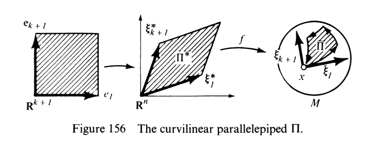
Given a manifold M. $\omega$ is a k-form defined on the tangent space of M at each point.

We pick a local coordinate system around $x \in M$ , so that there exists an open neighborhood $U \subset \mathbb{R}^n$ , containing 0, and a map $f$ that maps $U$ to a neighborhood of x. Let $\xi_1, ..., \xi_{k+1}$ be tangent vectors to M at point x. It follows that $df^{-1}(\xi_1) =: \xi_1', ... df^{-1}(\xi_n) =: \xi_n'$ lie in the tangent space to $\mathbb{R}^n$ at 0 (this space can be identified as $\mathbb{R}^n$ ).

Let $\Pi^{*}$ be the parallelepiped spanned by $\xi_1', ..., \xi_n' \in \mathbb{R}^n$ . We look at $f(\Pi^{*})$ which is a ‘curvilinear parallelpiped’ $\Pi$ on M. The boundary, $\partial{\Pi}$ , of $\Pi$ is a k-dimensional set. We consider the integral of the form $\omega^k$ on $\partial{\Pi}$ :

$F(\xi_1, ..., \xi_{k+1}) = \int_\partial{\Pi} \omega^k$

Physical interpretation: perhaps we can interpret this as finding the ‘flux’ of some kind of vector field across the boundary of the curvilinear parallelepiped?

How do we choose the k vectors for $\omega^k$ at each point?

Answer: we will need to parameterize the surface and then look at the tangent vectors corresponding to the parameterization at each point. But we will need to show that this remains invariant under bijective parameterizations.

Theorem: The principal (k+1)-linear part at 0 (not sure what Arnold meant by this, maybe at point x where we have defined the parallelepiped?) of the integral over the boundary of a curvilinear parallelepiped is unique and is a (k+1)-form, let’s call it $\Omega$ , i.e.

$F(\epsilon \xi_1, ..., \epsilon \xi_{k+1}) = \epsilon^{k+1} \Omega(\xi_1, ..., \xi_k+1) + o(\epsilon^{k+1})$ (as $\epsilon \rightarrow 0$ )

$\Omega$ is independent. of the choice of coordinates when used in defining F.

Suppose $x_1, ..., x_n$ are local coordinates on M and

$\omega^k = \sum a_{i_1, ..., i_k} dx_{i_1} \wedge ... \wedge dx_{i_k}$

(where the $a_{i_1, ..., i_k}$ ‘s are functions of $x_1, ..., x_n$ )

then it follows that

$\Omega = d\omega^k = \sum da_{i_1, ..., i_k} \wedge dx_{i_1} \wedge ... \wedge dx_{i_k}$ .

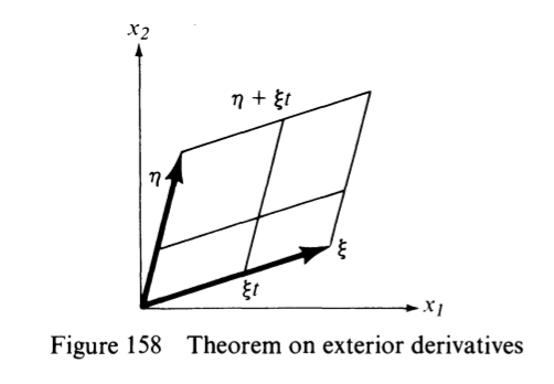
Let’s work through an example/proof for $\omega^1 = a(x_1, x_2)dx_1$ on the $(x_1, x_2)$ -plane.

Let $\Pi$ be the parallelogram with sides $\xi, \eta$ and vertex at 0. Then, $\partial{\Pi}$ can be parameterized (maps from $[0, 1] \rightarrow M$ ):

$t \mapsto \xi t$ (this has multiplicity 1)

$t \mapsto \eta t$ (multiplicity -1)

$t \mapsto \xi + \eta t$ (multiplicity 1)

$t \mapsto \eta + \xi t$ (multiplicity -1)

And so it follows that

$\int_{\partial{\Pi}} \omega^1 = \int_0^1 [a(\xi t) - a(\xi t + \eta)]dx_1(\xi) - [a(\eta t) - a(\eta t + \xi)]dx_1(\eta)$

Still thinking about:
Arnold claimed that:

$a(\xi t + \eta) - a(\xi t) = \frac{\partial{a}}{\partial x_1} dx_1(\eta) + \frac{\partial{a}}{\partial x_2}dx_2(\eta) + O(\xi^2, \eta^2)$

evaluated at $(x_1, x_2) = (0, 0)$

Similarly,

$a(\eta t + \xi) - a(\eta t) = \frac{\partial{a}}{\partial x_1} dx_1(\xi) + \frac{\partial{a}}{\partial x_2}dx_2(\xi) + O(\xi^2, \eta^2)$ .

How did he obtain these approximations?

Plugging these two expressions into the integral gives:

$F(\xi, \eta) = \frac{\partial a}{\partial x_2}(dx_2(\xi)dx_1(\eta) - dx_1(\xi)dx_2(\eta)) + o(\xi^2, \eta^2)$

The principal linear part of $latexF(\xi, \eta)$ is:

$\Omega = \frac{\partial{a}}{\partial x_2}dx_2 \wedge dx_1$ .

The expression we obtained also matches with the formula proposed in the theorem:

$da \wedge dx_1$

$= (\frac{\partial{a}}{\partial{x_1}} dx_1 + \frac{\partial{a}}{\partial{x_2}} dx_2) \wedge dx_1$

$= \frac{\partial{a}}{\partial x_2}dx_2 \wedge dx_1$

(this is because $dx_1 \wedge dx_1 = 0$ , i.e. the area of a 1-dimensional parallelogram is 0).

One response

Exterior Differentiation (Part 2) – Menagerie of Mathematics

September 24, 2025

[…] first part of the post is a continuation of the previous post Arnold’s Mathematical Methods of Classical Mechanics: Exterior Differentiation. The second part is based upon my reading of Lecture 1 of Arnold’s […]

LikeLike

Arnold’s Mathematical Methods of Classical Mechanics: Exterior Differentiation

Share this:

One response

Leave a Reply Cancel reply