Arnold’s Mathematical Methods of Classical Mechanics: the Geometry Behind Forms

This post is based upon my reading on the section on exterior forms in Arnold’s Mathematical Methods of Classical Mechanics.

Let $\mathbb{R}^n$ be an n-dim. vector space. We do not fix any special euclidean structure on $\mathbb{R}^n$ .

Definition of 1-form: It is a linear function $\omega : \mathbb{R}^n \rightarrow \mathbb{R}$ , i.e.

$\omega(\lambda_1 \xi_1 + \lambda_2 \xi_2) = \lambda_1 \omega(\xi_1) + \lambda_2 \omega(\xi_2)$ .

(where $\lambda_1, \lambda_2 \in \mathbb{R}, \xi_1, \xi_2 \in \mathbb{R}^n$ ).

The set of all 1-forms from $\mathbb{R}^n \rightarrow \mathbb{R}$ is a vector space, i.e.

$(\omega_1 + \omega_2)(\xi) = \omega_1(\xi) + \omega_2(\xi)$

$(\lambda \omega)(\xi) = \lambda \omega(\xi)$

(where $\lambda \in \mathbb{R}, \xi \in \mathbb{R}^n$ ).

Claim: the space of 1-forms on $\mathbb{R}^n$ is itself n-dimensional. It is called the dual space $(\mathbb{R}^n)^{*}$ .

Given $x_1, ..., x_n$ orthogonal coordinates in $\mathbb{R}^n$ , each coordinate $x_i$ is a 1-form, i.e.

$\omega_i : (x_1, ..., x_n) \mapsto x_i$

Geometrically, this is the projection of the vector onto the $x_i$ -axis, parallel in the other directions!

Given this basis of $\omega_i$ ‘s, every 1-form can be expressed as:

$\omega = a_1 x_1 + ... + a_n x_n$

The value of $\omega$ on a vector $\xi$ is:

$\omega(\xi) = a_1 x_1(\xi) + ... + a_n x_n(\xi)$

where $x_i(\xi)$ is the component of $\xi$ in the direction of $x_i$ .

Physical interpretation: let $\xi$ be the displacement vector and $(a_1, ..., a_n)$ be a uniform force field, $\mathcal{A}A$ , in $\mathbb{R}^n$ , then $\omega(\xi)$ is the work that $\mathcal{A}$ does on the displacement $\xi$ .

Geometric interpretation: $\omega(\xi)$ is the length of the projection of the vector $\xi$ onto the subspace spanned by $\mathcal{A} = (a_1, ..., a_n)$ (this projection is parallel along the other directions $\hat{N}_1, ... \hat{N}_{n-1}$ , where $\hat{N}_{\mathcal{A}} := \frac{\mathcal{A}}{|\mathcal{A}|}, \hat{N}_1, ..., \hat{N}_{n-1}$ form an orthonormal basis in $\mathbb{R}^n$ ).

Definition of 2-form: It is a bilinear and skew symmetric map $\omega^2 : \mathbb{R}^n \times \mathbb{R}^n \rightarrow \mathbb{R}$ , i.e.

$\omega^2(\lambda_1 \xi_1 + \lambda_2 \xi_2, \xi_3) = \lambda_1 \omega^2(\xi_1, \xi_3) + \lambda_2 \omega^2(\xi_2, \xi_3)$

$\omega^2(\xi_1, \xi_2) = - \omega^2(\xi_2, \xi_1)$

(where $\lambda_1, \lambda_2 \in \mathbb{R}, \xi_1, \xi_2, \xi_3 \in \mathbb{R}^n$ )

Examples of 2-forms:

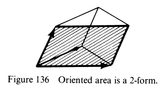
Example 1: Oriented area of parallelogram $S(\xi_1, \xi_2)$ in $\mathbb{R}^n$ .

Example 2: Oriented area of the projection of the parallelogram on the $x_1, x_2$ plane in $\mathbb{R}^3$ (given the coordinates of $\mathbb{R^3}$ are $x_1, x_2, x_3$ )

Figure taken from Arnold’s Mathematical Methods of Classical Mechanics.

Note: this is the 2-dimensional version of the projection we saw earlier. It is not difficult to see that the oriented area of the projection of parallelograms onto any plane in $\mathbb{R}^3$ (or in fact $\mathbb{R}^n$ ) gives us a 2-form, i.e., we can view the 2-forms as the oriented area of projections of 2-dimensional parallelograms onto a 2-dimensional subspace of $\mathbb{R}^n$ (with some choice of unit area)!

Example 3: in 3-dimensional oriented Euclidean space (the orientation gives us the skew-symmetry), the flux of the fluid (described by a constant field, say $\vec{v}$ ) over the area of the parallelogram $\xi_1, \xi_2$ given by:

$\omega^2(xi_1, xi_2) = (\vec{v}, \xi_1, \xi_2)$

where $(\vec{v}, \xi_1, \xi_2) = \vec{v} \cdot \hat{n} S(\xi_1, \xi_2)$ ( $\hat{x}$ is the unit vector normal to the parallelogram $S(\xi_1, \xi_2)$ and obtained from the right-hand rule).

Thinking about: can we interpret every 2 form as the flux of some sort of fluid field across the surface of a parallelogram?

It is now easy to see what $k-forms$ means.

Algebraically, it is a k-linear and anti-symmetric function of k vectors:

$\omega^k: \mathbb{R}^n \times ... \times \mathbb{R}^n \rightarrow \mathbb{R}$ .

Geometrically, it is the oriented volume of the projections of k-dimensional parallelepiped onto a k-dimensional subspace of $\mathbb{R}^n$ (with some choice in the unit volume).

Thus, an n-form in $\mathbb{R}^n$ gives us the volume of the parallelpiped up to a choice of unit volume.

Exterior Product of Two 1-forms

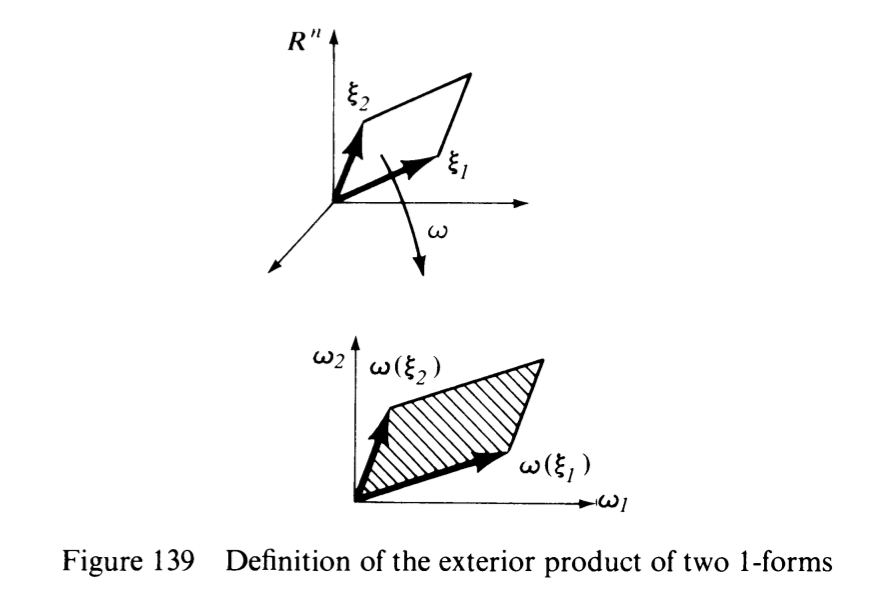
Given two 1-forms $\omega_1, \omega_2: \mathbb{R}^n \rightarrow \mathbb{R}$ , the exterior product of these two forms is a 2-form $\omega_1 \wedge \omega_2: \mathbb{R}^n \times \mathbb{R}^n \rightarrow \mathbb{R}$ defined in the most natural way

Algebraically, this is given by:

$(\xi_1, \xi_2) \mapsto \begin{vmatrix} \omega_1(\xi_1) & \omega_2(\xi_1) \\ \omega_1(\xi_2) & \omega_2(\xi_2) \end{vmatrix}$

it is easy to see using the properties of the determinant with respect to its rows that this map is bilinear and skew-symmetric.

Interesting observation: the map $(\omega_1, \omega_2) \mapsto \omega^1 \wedge \omega_2$ is also bilinear and skew-symmetric because the properties of the rows also hold for the columns.

Geometrically: $\omega_1, \omega_2$ is uniquely determined by vectors $\zeta_1, \zeta_2$ (maybe we can call them the characteristic vectors?). Recall, we can interpret a 1-form as the length of the projection of vectors onto a subspace spanned by another vector, say $\vec{w}$ . The $\zeta_1, \zeta_2$ are the respective $\vec{w}$ ‘s for $\omega_1, \omega_2$ . Notice that $\zeta_1, \zeta_2$ span a 2-dimensional plane. $(\omega_1(\xi_1) := \zeta_1 \cdot \xi_1, \omega_2(\xi_1) := \zeta_2 \cdot \xi_1)$ is the vector obtained from the projection of $\xi_1$ onto $(\zeta_1, \zeta_2)$ -plane, and $(\omega_1(\xi_2), \omega_2(\xi_2))$ is the vector obtained from the projection of $\xi_2$ onto $(\zeta_1, \zeta_2)$ -plane. Thus, $\omega_1 \wedge \omega_2 (\xi_1, \xi_2)$ gives us the oriented area of the parallelogram $\xi_1, \xi_2$ when projected onto the $(\zeta_1, \zeta_2)$ -plane!