June 7th: Harmonic Functions (Revisited)

This post is a reflection on a re-watching of the Harmonic Function video by Richard Borcherds. I had watched the video a couple of months ago, and watching it now, it is remarkable how refreshing I find it; I will try my best to share both my old and new interpretations.

Borcherds approach to harmonic functions is very complex analysis oriented (but of course), and so everything is in 2-dim. (which I find very concrete, and I’m also beginning to realize that restricting oneself to one specific dimension does not make things less exciting. In fact, this approach gives us plenty of diverse examples and thereby questions that we would have missed had we gone the general route. Say for instance, the tight connect between harmonic functions and complex analysis might be completely neglected if we had started off studying the solutions to the Laplacian equation in general n-dim. space.)

And so, in the perspective of complex analysis, it is interesting to ask:

When are smooth functions u defined in terms of x, y the real part of a holomorphic function w? (Note: if we want u to be the imaginary part of w, we simply rotate w on the plane by 90 degrees.)

We find by the Cauchy-Riemann equation that not all u would do; u needs to be harmonic.

Aside (example not in his video; can be found in Arnold’s PDE, section on double layers):

We examine $u(x, y) = \frac{x}{x^2 + y^2}$ on the plane. Claim: this is a harmonic function.

An intuitive explanation (very lacking in rigor):

We set the fundamental solution on the plane to be $u_0(r) = ln(\frac{1}{r})$ (coefficient is forgotten for simplicity; even Arnold did it in this case). Suppose we have a charge of +1 and -1 located a distance of $l$ apart on the x-axis with center of mass at the origin (and suppose the positive charge is on the LHS).

Then, it follows (by previous post) that the potential as $l$ goes to 0 is given by:

$u(r) = \frac{\partial ln(\frac{1}{r})}{\partial x_} = \frac{1}{r} \frac{\partial r}{\partial x_} = \frac{1}{r} (-\vec{x}, \nabla r) = \frac{1}{r} \frac{x}{r} = \frac{x}{x^2 + y^2}$ .

Key: $u(r)$ is really the limit of a difference 2 harmonic functions, so it makes sense that it is harmonic.

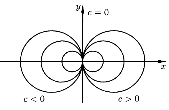
Notice that the level lines of this function are the family of circles tangent to the y-axis at the origin, because the level lines are $\frac{x}{x^2 + y^2} = c \Leftrightarrow x^2 + y^2 = cx$ .

Note: this function is not defined at the origin but well-defined everywhere else. So on a simply connected region not containing the origin, u is the real part of a holomorphic function w. How do we find the imaginary part?

Suppose v be the imaginary function of w, then the Cauchy Riemann equation gives:

$i \nabla u = \nabla v$ (learned from class; I like it much better than the real version. This one is much more geometrically useful. We can see that the level curves of these two functions are 90 degrees (clockwise) rotation of each other)

This tells us that the level curves of v are going to be the family of circles tangent to the x-axis at the origin.

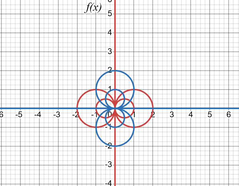
So from the level curves, we find that v is (up to a constant):

$\frac{y}{x^2+y^2}$ .

This means that $w(x, y) = \frac{x}{x^2 + y^2} + i\frac{y}{x^2+y^2} \Leftrightarrow w(z) = \frac{z}{z\bar{z}}$ , which is holomorphic when we stay away from the origin (notice that angles are preserved as this is really a ‘scaling’ function, where scaling is dependent of the location).

Returning back to Borcherds’ video:

Since the real and imaginary parts of holomorphic functions are harmonic, we can find the space of all harmonic polynomials in n=2 by taking the real and imaginary part of $z^n$ . We get:

${1, x, y, x^2-y^2, 2xy, ...}$ .

Claim: this is indeed a basis for the harmonic polynomials.

IIt is easy to see that the set we have is independent, thus it suffices to show that the dimension for each fixed degree of space of homogeneous harmonic polynomials is 2.

My approach from long ago (doesn’t work in higher dimension):

For given degree k. Suppose $x^k$ is a term in our polynomial p, then notice that $\Delta p$ will give us a term with $x^{k-2}$ . In order for that term to disappear, p must contain $x^{k-2}y^2$ since it is homogeneous. We can proceed to show that all terms of the form $x^{k-2m}y^{2m}$ must be contained in our polynomial (where k-2m >0). Notice that the terms of the form $x^{k-2m+1}y^{2m+1}$ is not necessary in our polynomial.

Similarly, we can show that if $x^{k+1}y$ is a term p, then p must contain all terms of the form $x^{k-2m+1}y^{2m+1}$ .

Hence, we have two degrees of freedom in constructing an independent set of homogeneous harmonic polynomial of degree k. Thus, the dimension is 2.

Now, I found out that this way of approaching is of no use in the general n-dim. case (for the 3-dim. case, it is already becoming very difficult). Showing that the laplacian taking the space of homogeneous harmonic polynomial of degree k to that of degree k-1 is surjective and then finding the dimension of the kernel is much more refined.

June 7th: Harmonic Functions (Revisited)

Share this:

Leave a Reply Cancel reply