June 1st: Solid Potential, Single-Layer Potential, Double-Layer Potential (Updated)

(Part 1) Reflection on solid potential and single layer potential:

Let $\Omega \subset \mathbb{R}^n$ be a bounded domain with charge density given by $f(x)$ . The physical interpretation of this would be a charged insulating solid with charge density given by $f(x)$ . We wish to find the potential at every point.

I recall from physics class that the elementary way of doing this would be to:

calculate/measure the electric field
compute the potential from that

But obviously, for a random solid, this does not seem like a good approach.

So instead of seeing $\Omega$ as one big solid, we think of it as a collection of point charges (this also appears to be a running theme in physics) and work with that instead, because we know the potential corresponding to a unit point charge is given by $u_0(x)$ where this is the fundamental solution in $\mathbb{R}^n$ . (Note: I can never remember the corresponding coefficient, but a nice thing to keep in mind is that the sign of the coefficient must be chosen so that $\Delta u_0(x)$ has positive value away from the origin. This is because the potential for a positive charge is positive.)

Key step:

$f(x) = \int_{\Omega} f(y) \delta_0(x-y)dy$

and the corresponding potential at $y$ with respect to $x \in \Omega$ is $f(x) u_0(x-y)$ . And so, the superposition of all these potentials at $y$ would give:

$u(y) = \int_{\Omega} f(x) u_0(x-y)dx$ .

Last time, my argument for showing $u(y)$ is harmonic had been:

$\Delta u(y) = \Delta \int_{\Omega} f(x) u_0(x-y)dx = \int_{\Omega} \Delta f(x) u_0(x-y)dx = \int_{\Omega} f(x) \delta(x-y)dx$ (this disappears for all $y \notin \Omega$ and equals to $f()$ for $y \in Omega$ ).

This is not even necessary if we consider $u(x)$ as a superposition of $f(x) u_0(x-y)$ . Everything just follows.

Single-Layer Potential

Here, we consider a charged surface instead of a solid. The physical interpretation is that of a charged conducting solid (all charges would be on the surface of the solid).

The potential is given similar to the above (except we change $\Omega$ to its boundary $\partial \Omega$ instead).

As above, potential is harmonic inside the region and outside. The interesting thing is on the boundary (the jump in the normal derivative is equal to $f$ , i.e. $\frac{\partial u}{\partial n_{+}} + \frac{\partial u}{\partial n_{-}} = f$ , where $f$ is the charge density). Proof for this had been given in a previous post. What I want to do here is understand this phenomenon through a few examples.

Recall: the example of the uniformly charged conducting sphere. The graph of the potential looks like:

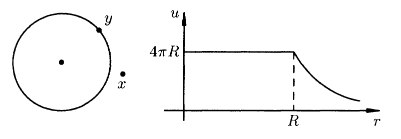
Due to the symmetry of the sphere, the potential at any point would only depend on the radial distance. Hence, it would be of the form $\frac{a}{r} + b$ . Since the potential inside the sphere must be harmonic (follows from above), this would mean that it is a constant inside the sphere. Key: it is easy for us to find the potential at the origin by superposition.Then the potential at the origin corresponding to each point (where the charge at the point is Q) on the sphere $\frac{Q}{4\pi \epsilon_0 R}$ . If the potential is $\frac{1}{R}$ , then the charge density would be $4\pi \epsilon_0$ .

Then, the potential at the origin would be:

$\int_{S^2} \frac{1}{R} dS = \frac{1}{R} 4\pi R^2 = 4\pi R$ .

And so, the potential at any point inside the sphere would be $4\pi R$ .

Outside, the potential is given by $u(r) = \frac{4\pi R^2}{r}$ (the value of a follows from continuity and the value of b=0 ensures the potential at infinity is 0).

In this example:

$\frac{\partial u}{\partial n_{+}}|_{r=R} = \frac{d}{dr}\frac{4\pi R^2}{r} = -4\pi$

$\frac{\partial u}{\partial n_{-}}|_{r=R} = \frac{d}{dr} 4\pi R = 0$

And so, $\frac{\partial u}{\partial n_{+}}|_{r=R} + \frac{\partial u}{\partial n_{-}}|_{r=R} = -4\pi$ (This is the charge density up to a coefficient).

Correction (curious why Arnold removed the $-\frac{1}{\epsilon_0}$ coefficient): $\frac{\partial u}{\partial n_{+}} + \frac{\partial u}{\partial n_{-}} = -\frac{f}{\epsilon_0}$ .

Double-Layer Potential

For some reason, I had (and still am) having a difficult time understanding the construction Arnold gave for the double-layer potential. I will write my interpretation below:

For simplicity, let’s restrict ourselves to $mathbb{R}^3$ , so a hypersurface in this case would be a 2-dim. surface (we assume to be smooth).

We now consider a charge distribution of 2 layers on a hypersurface, $S$ .

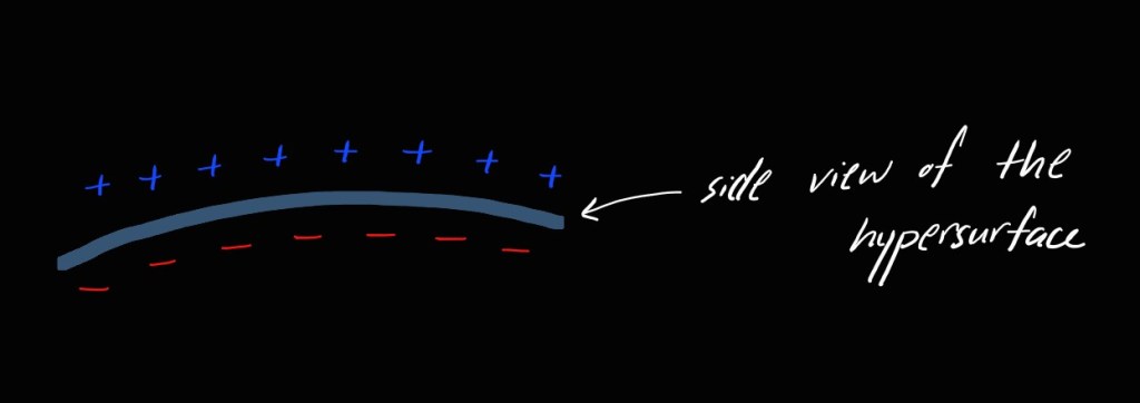
First confusion: Arnold said that this charge distribution can be described by a charge density $\rho(x)$ , where $\rho$ is a function on $S$ . Is he saying that the charge distribution for both layers is $\rho(x)$ at the ‘correspond’ point on $S$ ?

So that is what I have assumed moving forward.

Now, we look at the following (but be warned: certain things are still not making sense in my interpretation):

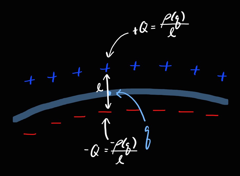
At point $q \in S$ , we draw a line normal to $S$ and let $l$ be the distance between the two layers of charges on that line (picture is above). But then, why on Earth would we say that the charge at $+Q = \frac{\rho(q)}{l}, -Q = -\frac{\rho(q)}{l}$ ?

I had a different interpretation (but not much better): we say that the charge density of the two layers combined at a corresponding point $x$ on $S$ is $\rho(x)$ , and then, at each point $x$ , we look at the charge density along the ‘thickness’ of the layer (i.e. the line that we had been describing), if we assume uniform charge density, then the charge at each point would be $\frac{\rho(x)}{l}$ . But the problem with this is that the two layers have opposite sign, assuming uniform charge implies that the net charge at point $x$ will be 0.

It doesn’t really make sense… But I’ll accept it.

So what will the potential corresponding to this point q be at a point x?

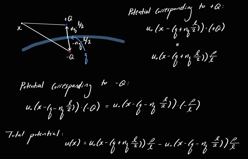
Notice that as $l \rightarrow 0$ , this (almost) is just:

$\rho \frac{\partial u_0(x-q)}{\partial n_q} + o(1)$ (*)(this is because $u_0$ away from the origin is smooth).

So the limit of this potential (for x away for the double layer) is a harmonic function (why? because the derivative of a harmonic function is still a harmonic function. Aside: it seems that the space of harmonic functions has some very nice structures. The entire space maps to itself under rotations, translations, dilations, addition/subtraction, and differentiation).

(*) gives us the potential of a dipole. Isn’t this nice?

Key: An electric dipole is the limit of the picture below. It is when the + and – charges become infinitely close together. If the two charges are of equal magnitude (which they are by definition), then the net charge is 0. But because of the structure, they create an electric field. In fact, the field somewhat resembles that of a magnetic field…

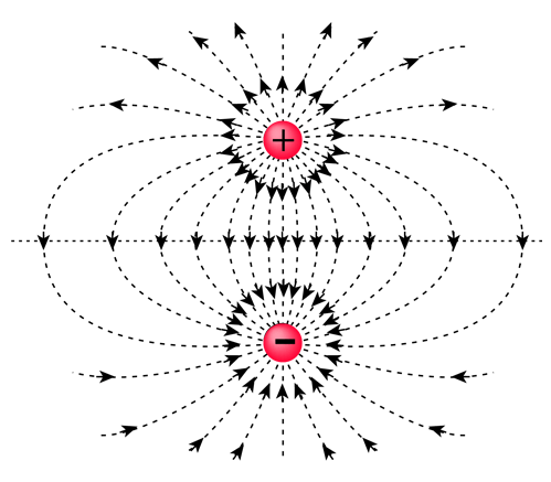
New interpretation: the double layer should really be considered as a surface of dipoles (this still does not explain the charge density that Arnold was talking about) and so the potential at x, by superposition, corresponding to the entire double layer would be:

$u(x) = \int_{S} \rho(q) \frac{\partial u_0(x-q)}{\partial n_q} dq$

Is this going to be easy to calculate for an arbitrary surface? Not really…

June 1st: Solid Potential, Single-Layer Potential, Double-Layer Potential (Updated)

Share this:

Leave a Reply Cancel reply