Monodromy Operator of a Linearized Periodic System: An Investigation

Feb 15—2025

This post is the second part of https://menagerieofmathematics.wordpress.com/2025/02/03/the-monodromy-operator/

and is based upon Problem 1 on p. 51 of Arnold’s ODE:

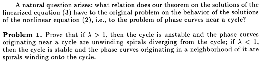
That is, we are interested in studying the relation between the behaviour of the solutions of the linearized equation to that of the solutions of the original equation.

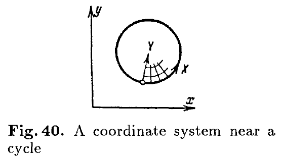
Recall, the original nonlinear equation that arose from the coordinate system depicted in the figure below is

$\frac{dY}{dX} = a(X, Y)$ (*) where $a(X, 0) = 0$ and $a(X + T, Y) = a(X, Y)$ .

We know that the solution with initial condition $(X=0, Y=0)$ is $Y=0$ .

For solutions of initial conditions $(0, \epsilon)$ (for $\epsilon$ small), they can be expressed as

$\phi(X) = \phi_0(X) + \phi_1(X)\epsilon + \phi_2(X)\epsilon^2 + ...$ (where the … represents the terms of order higher than 2)

Since for $\epsilon = 0$ , $\phi(X) = 0$ , it follows that $\phi_0(X) = 0$ .

Since $\phi(0) = \epsilon$ , $\phi_1(0) = 1$ and $\phi_k(0) = 0$ for all $k \geq 2$ .

The return function for equation (*) is by definition

$\Phi: \phi(0) = \epsilon \rightarrow \phi(T) = \phi_1(T)\epsilon + \phi_2(T)\epsilon^2 + ...$

i.e. $\Phi(\epsilon) = \phi_1(T)\epsilon + \phi_2(T)\epsilon^2 + ...$ .

Thus, the linearization of the return function in Y at $Y = 0$ would give us the operator

$\Phi_{*}(\epsilon) = \Phi'(0) \epsilon = \phi_1(T)\epsilon$ .

It is easy to see that this is a monodromy operator.

Recall: $\Phi'(0) > 1$ implies the cycle is unstable and nearby phase curves diverge. $\Phi'(0) < 1$ implies the cycle is stable and nearby phase curves converge.

Thus, it suffices to study the value of $\phi_1(T)$ . How do we determine this value if we know the linearized version of equation (*) (i.e. $\frac{dY}{dX} = f(X)Y$ where $f(X) = \frac{\partial a}{\partial Y}|_{Y=0}$ )?

For Y small, we can approximate $a(X, Y)$ with its Taylor expansion in Y:

$a(X, Y) = \frac{\partial a}{\partial Y}|_{Y=0} \cdot Y + \frac{\frac{\partial^2 a}{\partial Y^2}|_{Y=0} \cdot Y^2}{2!} + ...$

Hence, (*) would become:

$\frac{dY}{dX} = \frac{\partial a}{\partial Y}|_{Y=0} \cdot Y + \frac{\frac{\partial^2 a}{\partial Y^2}|_{Y=0} \cdot Y^2}{2!} + ...$

Substituting the general solution $\phi(X) = \phi_0(X) + \phi_1(X)\epsilon + \phi_2(X)\epsilon^2 + ...$ into the above and taking the equation for the first order gives:

$\frac{d\phi_1(X)}{dX} = \frac{\partial a}{\partial Y}|_{Y=0} \cdot \phi_1(X) = f(X) \phi_1(X)$ (**).

Rearranging (**) gives:

$\frac{1}{\phi_1(X)}d\phi_1(X) = f(X)dX$

Integrating both side of the above equation from 0 to T gives:

$ln(\phi_1(T)) - ln\phi_1(0)) = \int_0^T f(X)dX$ .

Since $\phi_1(0) = 1$ , it follows that the above could be simplified to:

$\phi_1(T) = e^{\int_0^T f(X)dX} = \lambda$ , where $\lambda$ is by definition the multiplier of the monodromy operator of the linearized equation.

Hence, when $\Phi'(0) = \phi_1(T) = \lambda < 1$ , the cycle is stable and when $\Phi'(0) = \phi_1(T) = \lambda > 1$ , the cycle is unstable. When $\Phi'(0) = \phi_1(T) = \lambda = 1$ , we cannot determine the exact behaviour of the phase curves around the cycle.