The Monodromy Operator (Part 1)

The first time reading through Arnold’s ODE, I had thought that the Section on linear equations he had placed in between Section 2: Vector Fields on the Line and Section 4: Phase Flows was awkward; it felt disruptive to the flow of the book.

That was because I had not been paying much attention to a special something that had been re-appearing again and again in the sections: the monodromy operator.

It first occurred in the Lotka-Volterra model and was used to study the behaviours of limit cycles. More on that in my previous post: https://menagerieofmathematics.wordpress.com/2025/01/30/a-re-understanding-of-the-return-function/.

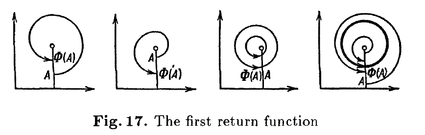
The key idea is to look at the changes of the y-value given a fixed x-value on the phase curves. The notion of periodicity is subtle; how can we see it?

This is what Section 3: Linear Equations build upon:

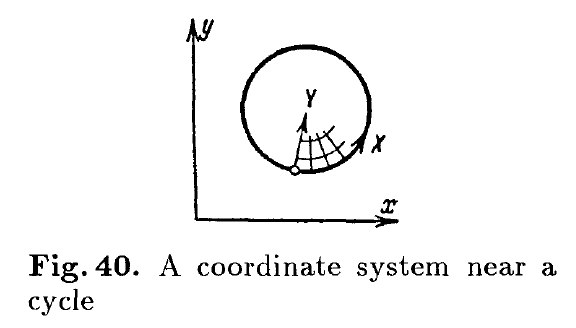
Periodicity is relative; we need an object of reference. In systems with closed cycles, periodicity is relative to the cycle. Looking at the above figure, we construct a local coordinate system on the cycle; we set X to be on the cycle and Y to be a transversal of the cycle (it follows that Y = 0 is the cycle). Then locally, the coordinates will be (X mod T, Y), where T is one traversal around the cycle.

The phase curves nearby can be seen as integral curves of the equation:

$\frac{dX}{dY} = a(X, Y)$ where $a(X, 0) = 0$ and $a(X, Y) \equiv a(X+T, Y)$ .

Important step: linearization of the above in terms of Y at Y = 0 gives

$\frac{dX}{dY} = f(X)Y$ where $f(X) = \frac{\partial a}{\partial Y}|_{Y=0}$ (Note, this is homogeneous because $a(X, 0) = 0$ .)

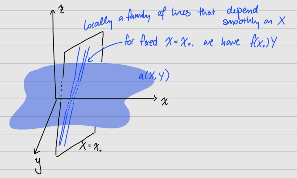
Geometrically, the linearization in Y represents a family of lines that depend smoothly on the change in X. For a fixed $X = X_0$ , the linearization gives us the line $f(X_0)Y$ . Hence in a neighbourhood of (X₀, 0), the graph of this linearization is the set of lines $f(X)Y$ for X near $X_0$.

Now, it suffices for us to study linear homogeneous equations with periodic coefficients, i.e.

$\frac{dX}{dY} = f(X)Y$ where $f(X + T) \equiv f(X)$

Enter: the monodromy operator

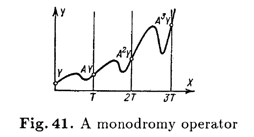
The mapping $A: R \rightarrow R$ maps the value $\phi(0)$ to the corresponding value $\phi(T)$ .

Notice:

The direction field is invariant under translation by T along the X-axis (i.e. the direction field is T-periodic along the X-axis) and so, the integral curves map to each other under translations by T.
The direction field is invariant under dilation along the Y-axis (due to the fact that this is a homogeneous equation). Hence, integral curves map to each other under dilations.

What does these two properties imply?

The integral curve passing through the point $(T, \phi(T))$ is a translation of the dilated integral curve passing through the point $(0, \phi(0))$ . We can see this in Fig. 41 as well. Notice that the section of the integral curve between T and 2T is a dilation of the section between 0 and T, and so on so forth…

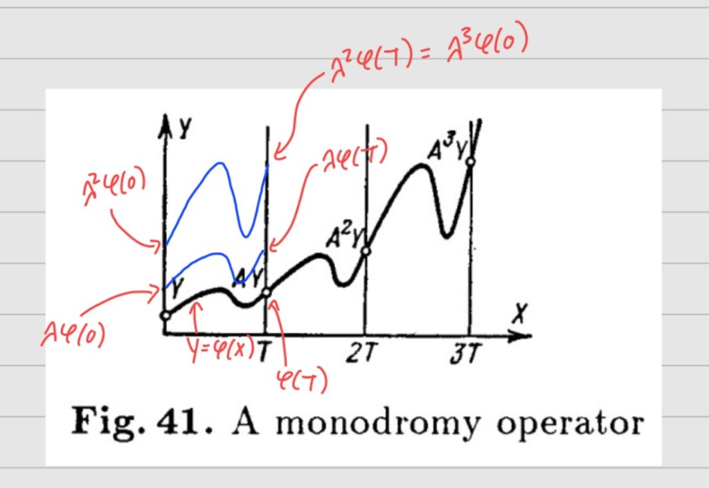
Claim: dilation at each section is by the same amount, i.e. $\phi(X + T) = A(\phi(X)) = \lambda\phi(X)$ (the monodromy operator is linear).

Intuitively, we can wrap this direction field around a cylinder of circumference T so that the sections of an integral curve $\phi(X)$ coincide (are on top of) the dilated $\phi(X)$ beginning at X = 0.

$\phi(T) = A(\phi(0)) = \lambda\phi(0)$ by some constant $\lambda$

$\phi(2T) = A(\phi(T)) = \lambda \cdot \lambda\phi(0) = \lambda^2 \phi(0)$

$\phi(3T) = ... = \lambda^n\phi(0)$

Hence, it follows that the monodromy operator is linear.

In general, $\phi(nT + X_0) = \lambda^n \phi(X_0)$ . Why? Because the integral curve passing through this point $(nT + X_0, \phi(nT + X_0)$ is a translation by nT of the integral curve $\lambda^n \phi(X)$ with initial condition $(0, \phi(0))$ . Thus, $(nT + X_0, \phi(nT + X_0)$ is the translation of the point $(X_0, \lambda^n \phi(X_0)$ by nT.