A Different Approach: Perturbation Method (Variant of Newton’s Series Method)

In my previous post (https://menagerieofmathematics.wordpress.com/2025/01/28/rectification-theorem-dependence-on-initial-condition-newtons-method-and-an-example/), we discussed the local smooth dependence of solution on its initial condition; this follows from the rectification theorem.

In this post, we will look at the application of this result. What is the significance behind the smooth dependence of solution on its initial condition?

Given $\dot x = v(t, x)$ (2nd order ODEs could also work cf. Problem 3 of this post) with a smooth RHS, if we are able to find an initial condition $(t_0, x_0)$ with a special solution, then we can approximate (first order) solutions of nearby initial conditions. This is the underlying idea of the perturbation method that we will be exploring through specific examples.

All problems in this post are taken from p. 94 and 95 of Arnold’s ODE.

Notice that the solution of $\dot x = x^2 + x \cdot sin(t)$ with the initial condition $(0, 0)$ is $\phi_0(t) = 0$ .

For integral curves of initial conditions $(0, a)$ (for $a$ small), they depend smoothly on $a$ . Hence, we can Taylor expand them in terms of $a$ at $a = 0$ :

$\phi(t) = \phi_0(t) + \phi_1(t) \cdot a + o(a^2)$ (*)

(Note: we are only interested in approximating the solutions up to the first order. Since for $a$ small, higher orders contribute insignificantly.)

So far, we know:

$\phi_0(t) = 0$ (1) and

$\phi(0) = a$ (2).

From (2), it follows that $\phi_1(0) = 1$ .

And substituting (*) into the ODE gives:

$\dot{\phi_1}(t) \cdot a + o(a^2) = (\phi_1(t) + o(a^2))^2 +(\phi_1(t) + o(a^2)) \cdot sin(t)$

Since we only care about the o(a) terms, the above approximates to:

$\dot{\phi_1}(t) = \phi_1(t) \cdot sin(t)$ (**), which is a homogeneous linear equation.

The solution with the initial condition $(0, 1)$ that satisfies the above (**) is $\phi_1(t) = e^{1-cos(t)}$. This is the derivative that we have been searching for.

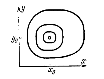
Recall, the phase curves of the Lotka-Volterra system are closed and are only defined for $x \geq 0$ and $y \geq 0$ .

The phase curve with the initial condition $(1, 0)$ is $y_0(x) = 0$ . (Why? because at the initial condition, the velocity vector in the y-direction is $dy(A) = 0 \cdot (1 - 1)$ ; hence, the particle never leaves the x-axis.)

Since the field is smooth, phase curves of initial conditions $(1, \epsilon)$ for $\epsilon$ small can be locally expressed as:

$y(x) = y_0(x) + \epsilon \cdot y_1(x) + o(\epsilon^2)$ (*)

Notice, since we are approximating with error of $\epsilon^2$ , the differential equations can be approximated to:

$\dot x = x(1 -ya(x,y)) \approx x$

$\dot y = y(x - 1)$ .

Important shift in POV: the phase curves (approx.) coincide with the integral curves of

$\frac{dy}{dx} = \frac{y(x-1)}{x}$

Substituting (*) into the above gives:

$\dot{y_1}(x) \cdot \epsilon + o(\epsilon^2) = \frac{(\epsilon \cdot y_1(x) + o(\epsilon^2))(x-1)}{x}$ .

The first-order equation that follows is:

$\dot{y_1}(x) = y_1(x)(1 - \frac{1}{x})$ , a homogeneous linear equation.

The solution for the above equation that satisfies the initial condition $y_1(1) = 1$ (because we want $y(1) = \epsilon$ ) is $y = \epsilon \cdot \frac{e^{x-1}}{x}$ .

Important: $\theta(0) = a$ tells us the angle of the pendulum at $t = 0$ and the fact that $\dot{\theta}(0) = 0$ tells us that the pendulum is starting at rest. This means, $\theta = a$ is the largest angle that the pendulum could reach (i.e. $- a \leq \theta \leq a$ ), and so for $a$ small, $\theta$ is also small for all time.

Why is this important?

We know that for $\theta$ small, $sin(\theta) \approx \theta$

(Note: order of error will be $o(a^3)$ because of the Taylor series of sine, $sin(\theta) = \theta - \frac{\theta^3}{3!} + ... = \theta + o(\theta^3)$ ).