Differential Equations on Manifolds: Part 2 (15/09/2025)

In this post, we explore the notion of compactness and connectedness for manifolds. This is based upon my reading of Chapter 5: Differential Equations on Manifolds in Arnold’s ODE.

Compactness

Sets in $\mathbb{R}^n$ are compact if for any open covering, there exists a finite sub-covering. So it makes sense to extend this definition to manifolds.

But, how do we define open sets on manifolds?

We use the charts that gave our manifolds the ‘differentiable structure’.

Definition of open set: $G \subset M$ is open if on any chart $(W_i, \phi_i)$ , $\phi_i(G \cap W_i)$ is open.

We can show that finite intersections of open sets and unions of any number of open sets are open, but since the goal of this post is to work through some interesting problems and examples that involve these concepts, I will not write out the proofs here.

Definition of compact set: $K \subset M$ is compact if every covering of it by open subsets contains a finite sub covering.

Problem 1: Prove that the sphere $S^n$ is compact.

Let’s first look at the case of when n = 2.

Consider:

$F_1 = \text{upper semi-sphere} \cup \text{equator parallel to the (x,y)-plane}$

$F_2 = \text{lower semi-sphere} \cup \text{equator parallel to the (x, y)-plane}$

(Note: $F_1 \cup F_2 = S^2$ )

$\phi_1$ be the stereographic projection from the North Pole,

and $\phi_2$ be the stereographic projection from the South Pole.

It is not difficult to see that $\phi_2(F_1) = \overline{\mathbb{D}} = \phi_1(F_2)$ (where $\overline{\mathbb{D}}$ is the unit disk with its boundary). This is a compact set in $\mathbb{R}^2$ .

Given an open covering of $S^2$ , say $\{G_k \}_{k \in K}$ . Then, $\{ \phi_1(G_k) \}_{k \in K}$ is an open covering of $\overline{\mathbb{D}}$ . Since $\overline{\mathbb{D}}$ is compact, we can find a finite subset $K' \subset K$ such that $\{ \phi_1{G_k'} \}_{k' in K'}$ is a sub-covering. Since $\phi_1$ is a bijection, it follows that $\{ G_k' \}_{k' \in K'}$ is a finite sub covering for $F_1$ .

Similarly, we can find a finite sub-covering for $F_2$ . The union of these two finite sub-covering gives us a finite sub covering for $S^2$ .

This proof holds for any higher $n \in \mathbb{N}$ ; the only difference would be that the image of the stereographic projection for the semi-n-sphere with its equator would be the $n-1$ ball with its boundary, which is also compact.

Problem 2: Is the projective space $\mathbb{RP}^n$ compact?

For simplicity, we examine the case of when $n=1$ . This would be the space of lines passing through the origin in $\mathbb{R}^3$ .

Consider:

$A_1 = \{ [x_0 : x_1] | x_0 \neq 0, |x_0| \leq |x_1| \}$

$B_1 = \{ [x_0 : x_1] | x_0 \neq 0, |x_0| \geq |x_1| \}$

$B_2 = \{ [x_0 : x_1] | x_1 \neq 0, |x_1| \leq |x_0| \}$

$A_2 = \{ [x_0 : x_1] | x_1 \neq 0, |x_1| \geq |x_0| \}$

(Note: $latex A_1 \cup B_1 \cup A_2 \cup B_2 = \mathbb{RP}^1)

and the following two maps:

$\phi_A: [x_0 : x_1] \rightarrow \frac{x_0}{x_1}$

$\phi_B: [x_0 : x_1] \rightarrow \frac{x_1}{x_0}$ .

It is not difficult to see that $\phi_A(A_1), \phi_A(A_2), \phi_B(B_1), \phi_B(B_2) = [-1, 1]$ , which is compact.

(Looking at my solution now: two of the sets are not needed. Which are they? When we are considering, say $x_0 \neq 0$ , it suffices to only consider the case $|x_1| \leq |x_0|$ . The other case would be a subset of { $x_1 \neq 0$ and $|x_0| \leq |x_1|$ }.

We can then apply the same argument as we did in the first problem to show that $\mathbb{RP}^1$ is compact.

For higher dimensions, the proof would be similar. We would need to consider all the cases that would cover $\mathbb{RP}^n$ .

For instance, for $\mathbb{RP}^2$ . The subsets we consider are:

$A = \{ [x_0, x_1, x_2] | x_0 \neq 0, |x_1| \leq |x_0|, |x_2| \leq |x_0| \}$

$B = \{ [x_0, x_1, x_2] | x_1 \neq 0, |x_0| \leq |x_1|, |x_2| \leq |x_1| \}$

$C = \{ [x_0, x_1, x_2] | x_2 \neq 0, |x_0| \leq |x_2|, |x_1| \leq |x_2| \}$

(there are no additional cases we need to consider. For instance, $\{ [x_0, x_1, x_2] | x_0 \neq 0, |x_1| \leq |x_0|, |x_2| \geq |x_0| \}$ would be a subset of $C$ . We have $A \cup B \cup C = \mathbb{RP}^2$ .)

The image of the sets under the maps would be the (n-1)-dimensional solid unit cube.

Connectedness

The image that Arnold has put inside the book perfectly shows what it means for a manifold to be connected:

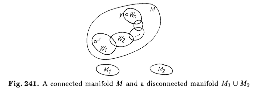
In words, we say M is connected if given any 2 points $x, y \in M$ , there exists a finite chain of charts $(W_i, \phi_i)$ such that $x \in W_1$ and $y \in W_n$ and $W_i \cap W_{i+1} \neq \emptyset$ AND $\phi_i(W_i)$ is connected.

Problem 3: Is the following manifold connected in $\mathbb{R}^3$ (in $\mathbb{RP}^3$ ):

$x^2 - y^2 - z^2 = C$ ( $C \neq 0$ )?

When C > 0, we obtain a two-sheeted hyperboloid in $\mathbb{R}^3$ . Hence, the surface is not connected.

Suppose C = 1. Then the two points with minimum absolute x-value are: (-1, 0, 0) and (1, 0, 0). There does not exist any points with smaller absolute x-values. Hence, these two points are not connected.

When C < 0, we obtain a one-sheeted hyperboloid. This surface is connected.

Aside: I used Desmos to help me visualize the surfaces. But is it possible to determine if 3-dim. quadric surfaces are connected without drawing the surface out?

Note: this equation is not well-defined in $\mathbb{RP}^3$ . We would need to homogenize it:

$x^2 - y^2 - z^2 = Cw^2$

Still thinking about: how do we determine the number of connected components of this curve? In $\mathbb{RP}^2$ , we have Harnack’s theorem.

Problem 4: The set of all matrices of order n having nonzero determinant has a natural differentiable manifold structure (a domain in $\mathbb{R}^{n^2}$ ). How many connected components does this manifold have?

The natural differentiable manifold structure arises from the following map (I will use n = 2 for simplicity of writing):

$\begin{bmatrix} a_{11} & a_{12} \\ a_{21} & a_{22} \end{bmatrix} \rightarrow (a_{11}, a_{12}, a_{21}, a_{22})$

The image of the set of non-invertible matrices is given by:

$\{ (x_{11}, ..., x_{1n}, x_{21}, ...., x_{nn}) | P(x_{11}, ..., x_{1n}, x_{21}, ...., x_{nn}) = 0, \text{where P is the characteristic polynomial} \}$

Any other point in $\mathbb{R}^{n^2}$ corresponds uniquely to an invertible matrix.

In the n = 2 case, the image of the set of non-invertible matrices is:

$\{ (x_{11}, x_{12}, x_{21}, x_{22}) | x_{11}x_{22} - x_{12}x_{21} = 0 \}$

Since $x_{11}x_{22} – x_{12}x_{21} = 0$ is a smooth surface of dimension-3 in $\mathbb{R}^4$ , it is not difficult to see (although I am not sure how to rigorously prove this) that this surface partitions $\mathbb{R}^4$ into 2 components.

We can give the same argument for any higher n.

So, what are the two components?

Key: geometrically, the image of the set of non-invertible matrices is the zero set of the characteristic polynomial. It partitions the set of level surfaces into the positive and negative, i.e. on one side, we would have the level surfaces for $P = \text{positive constant}$ and on the other side, we would have the level surfaces for $P = \text{negative constant}$ . Hence, the two components of the $GL_n(\mathbb{R})$ are the set of matrices with positive determinant and the set of matrices with negative determinant.

Differential Equations on Manifolds: Part 2 (15/09/2025)

Share this:

Leave a Reply Cancel reply