In this post, we will be focusing on the theorem of removable singularities for harmonic functions on the plane:

and its applications.

Arnold gave a physical interpretation of this theorem that I find interesting. Harmonic functions describe the steady-state position of a thin sheet stretched over some curve. The curve in this case would be the boundary of the neighbourhood. If the surface formed by the sheet is indeed in steady-state except at one point, then we can by continuity, figure out the position of the surface at that point so that the entire surface is still in steady-state. Recall: harmonic functions do not attain maximum value on the interior of a region. Hence, a surface obtained by propping up the sheet at one point inside the circle cannot possibly be in steady-state:
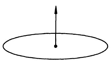
We can also verify this physically. If we are to prop our stretched sheet at one point with a very thin needle, the needle will go right through.

Aside: Arnold mentioned that the steady state of a very thin plate, which is described by \Delta^2 u = 0, can indeed achieved by propping the plate up at one point by a thin needle. This is quite interesting, and to better understand this, I will need to look more into the solutions of this equation, which I think is called the biharmonic equation. Since harmonic functions on the plane are closely related to holomorphic functions, it will be interesting to figure out the relationship between biharmonic functions and holomorphic functions.

So now, without further ado, let’s jump into the proof.

Let’s suppose the region we are concerned with is the unit disk centered at 0, and the bounded harmonic function, f, is defined everywhere inside the circle except at point 0.

We can find (will be proven in a following post) a harmonic function, h, defined inside and on the boundary of the disk and that coincides with f on the boundary. Let u = h - f. We wish to show that u = 0 on the entire punctured disk, this then tells us that h is the extension of f we are looking for.

The method that Arnold used to show u = 0 is called the barrier method. Let’s see why it’s named this way.

Consider u_0(r) = C ln(1/r). It is a harmonic function defined on the punctured disk and is 0 on the boundary. Key: since u is bounded (because f and h are bounded), we can choose a C so that u_0 geq u. In particular, we want to sandwich u between 0 and a family of u_0‘s that converge pointwise to 0.

Let M \geq |u| on the entire punctured disk. Suppose we want to construct u_0 such that it is equal to M on the circle with radius $latex\epsilon << 1$. Then, it suffices to choose C = \frac{M}{ln(1/\epsilon)}.

Notice that u_0 - u is harmonic on the annulus defined by r = 1, \epsilon, and since u_0 - u are non-negative on both the circle defined by r = 1 and that defined by r = \epsilon, u_0 - u cannot be negative inside the annulus. Hence, u \leq u_0 inside the annulus.

Arnold then claimed that:

0 \leq u \leq u_0 = \frac{m}{ln(1/\epsilon)}ln(1/r) (*) on the entire disk.

But how do we know u \geq 0? Why can’t u be negative inside the annulus? To answer this question, we need to ask: is it possible for u to attain both negative and positive values in the annulus?

Notice that as \epsilon \rightarrow 0, the RHS of (*), defined on the annulus bounded between \epsilon < r < 1, also goes to 0 (on a region of the annulus bounded between \epsilon + \delta < r < 1 for some \delta > 0; the convergence to 0 is quite slow). This forces u = 0 on the punctured disk.

Here are 2 drawings in the book that allows one to really see the ‘barrier’ formed at r = \epsilon.
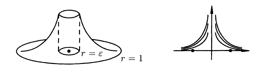
As \epsilon \rightarrow 0, notice that the u_0 function slowly collapses to 0.

My thoughts: I’m still not sure why we can assume u to be non-negative. If we do not assume this on u, then we would have:

\frac{M}{ln(\epsilon)}ln(1/r) \leq u \leq \frac{M}{ln(1/\epsilon)}ln(1/r) and as \epsilon \rightarrow 0, this would go to 0.

Leave a Reply

Is this your new site? Log in to activate admin features and dismiss this message
Log In