We left off last time (May 9th) after finding the fundamental solution to \Delta u = \delta(x) in \mathbb{R}^n. Recall: the solution is u_0(x) = \frac{1}{(2-n) \omega_{n-1} r^{n-2}} (where \omega_{n-1} is the surface area of the unit sphere in S^{n}).

Goal for this post: explore the physical significances behind this fundamental solution.

We begin by exploring \Delta \frac{1}{r^{n-2}} in the entire \mathbb{R}^n, but for simplicity, we will restrict ourselves to n = 3.

We know from before that when r \neq 0, \Delta \frac{1}{r} = 0. So what about at the origin?

Notice that the flux across the surface of any sphere is -4\pi. This follows from the fact that grad(\frac{1}{r}) is in opposite direction of the normal vectors pointing outward of the surface of the sphere and the magnitude of grad(\frac{1}{r}) at each point on the surface is \frac{1}{r^2}. Since the surface area of the sphere is 4\pi r^2, it follows that the total flux across the surface is - 4\pi (if we take the direction of the normal vector pointing outwards to be positive). This is true for any sphere centered at the origin. We can extend this statement to any closed surface containing the origin. Why?

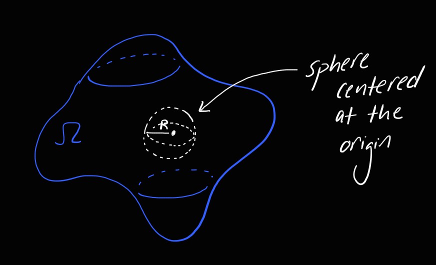
Explanation: Let’s call our chosen closed surface containing the origin \Omega. Find a sphere S of radius $\latex r$ that is completely contained in \Omega. We consider the flux across the region lying between the S and \Omega. Since \Delta u = 0 at all points not the origin, by the Divergence Theorem, it follows that the flux across this region must be 0. This means that the flux across the surface of \Omega must cancel out with the flux across the surface of S. We have what we want.

Region within \Omega where the flux is 0.

We can make such closed surface arbitrarily small, as long as it contains the origin. What does this say about \Delta u?

  • \Delta u = 0 for all x \neq 0
  • \int_{\Omega}\Delta u dV = -4\pi for all \Omega containing the origin

Does this make us remember something? Yes, the \delta-function! By definition, \Delta u = -4\pi \delta(x).

Physical meaning of the fundamental solution, u: this represents the potential of a unit charge at 0. In the case for n = 3, u_0 = -\frac{1}{4\pi r}.

A minor question: the potential corresponding to a positive charge should be non-negative, so are we assuming that this unit charge is a negative charge?

A nice change of view:
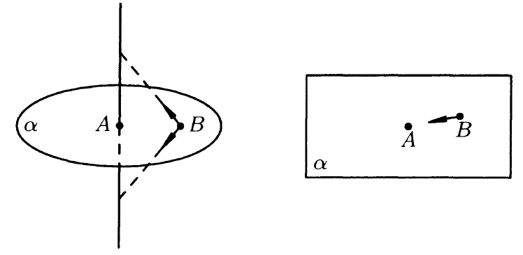
p. 91 of Arnold’s PDE

Key: we can go back and forth between potentials and fields.

The above diagram gives us a way of understanding electric fields on the plane as a “slice” of the electric field of a uniformly charged line in 3D.

We can compute the potential at point B in 2 ways:

  1. Find the electric field created by the line at point B and then compute the potential. Classic 🙂
  2. (slightly sketchy) We consider the picture to the right and restrict everything to the plane passing perpendicular to the line at A. We put the “entire” charge at point A (note: this is the weird part. The total charge on the line might be infinite. How can we put that all at A? Maybe I’m understanding this completely wrong…) and compute things on the plane.

Anyhow, Arnold warns us not to “add” all the potentials corresponding to each point. He then proceeds to give this formula:
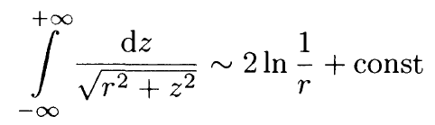
This is certainly remarkable, given the LHS does not even converge. The RHS is the computation restricted onto the plane and the LHS (not too sure) is what happens when you “add” the potential corresponding to each point along the line.

So how do we compute the potential associated to a region of charge and not just a point charge?

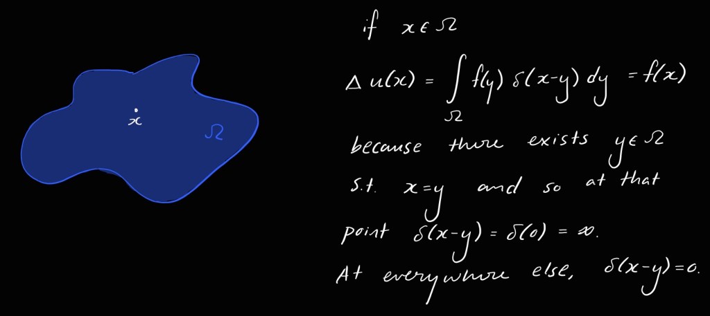
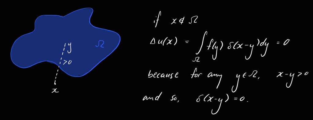
Suppose on a region \Omega, at each point y \in \Omega, there is a charge of magnitude f(y), then the potential that this charge creates at a point x is: u_0(x-y)f(y) (u_0 = \frac{1}{(2-n) \omega_{n-1} r^{n-2}}). Aside: this solution is just simply a shift and scaled version of the original solution; where the initial solution reaches \infty at the origin, here it reaches \infty at y (this makes sense since the charge we are now considering is at y). The potential corresponding to a charge at a fixed radius is also directly proportional to the magnitude of the charge, hence, this explains why it suffices to scale u_0 by f(y).

A minor question: Why do we take f(y) to be the magnitude of the charge? How would we then represent negative charges?

Then, by superposition, it follows that at point x, the potential corresponding to \Omega would be:

u(x) = \int_{\Omega} f(y)\u_0(x-y)dy.

Then,

\Delta u = \int_{\Omega} f(y) \delta(x-y) dy (assuming we can take derivative inside the integral).

Very sketchy thinking

It follows that \Delta u(x) = f(x) in the region and is harmonic outside.

What about uniqueness of this solution u(x)? It is up to adding by any harmonic function.

But if we impose the condition that at infinity, u(x) vanishes, then we have uniqueness (this follows from the maximum principle). What about when n = 2? Recall the fundamental solution is a scalar multiple of log(x). In this case, uniqueness is up to an addition of a constant and the condition we impose to obtain such uniqueness is for the solution to be bounded by logarithmic growth as x tends to infinity, i.e. |u(x)| \leq |klog(x)| (for some k).

This is a very interesting phenomenon: harmonic functions on the plane whose growth is bounded by a logarithm must be constant. (Why?)

Leave a Reply

Is this your new site? Log in to activate admin features and dismiss this message
Log In